10.1 Two centuries in one book

The methods of the preceding chapters were presented in the order that makes them easiest to learn, which is not the order in which they were invented. Restoring the chronology is worth a few pages, because almost every technique in this book was a response to a specific failure of the one before it, and that lineage explains both what each method does well and what it was never meant to do.

10.1.1 From least squares to the probability approach

Everything starts in 1805, when Legendre publishes the method of least squares, followed by Gauss in 1809, who adds the probabilistic justification: if the errors are normal, the least squares estimate is the most probable one. The tool exists before the theory that explains it, which will happen again more than once in this book.

The word regression arrives in 1886, and by accident. Galton, studying the height of children against that of their parents, observes that tall parents have children who are on average shorter than themselves, and names the phenomenon regression towards mediocrity. He was describing a property of the data, not a method; the name stuck to the method.

The first third of the twentieth century is Fisher’s. Maximum likelihood, the analysis of variance, the design of experiments, the distributions that carry his name and Student’s: what our chapters two to five present as routine is the residue of that period, and the assumptions we tested there are the ones he made explicit.

Econometrics separates itself in the nineteen thirties, with the founding of the Econometric Society in 1930 and Frisch’s programme of uniting theory, mathematics and statistics. The decisive text is Haavelmo’s, in 1944: economic data are not experiments, they are one realization of a stochastic process, and the whole apparatus of statistical inference can be applied to them only if that is stated explicitly. Everything our chapters on the assumptions are about descends from that paper.

10.1.2 The econometric synthesis

The next forty years build the discipline as it is still taught. The Cowles Commission formalizes simultaneous equations and the identification problem, which we met in the structural form of the VAR. The assumptions are examined one by one, and each violation gets its remedy: heteroskedasticity, autocorrelation, endogeneity, and the instrumental variables that answer it.

Time series become a field of their own with Box and Jenkins in 1970, whose four-step methodology we followed in chapter seven. Then comes a series of results that changed applied practice completely. Granger and Newbold show in 1974 that regressing two independent random walks produces a spurious relation with an excellent \(R^2\), which invalidated a good part of the published work of the time. Dickey and Fuller give the test for it in 1979. Engle introduces ARCH in 1982 to model a variance that changes over time, Bollerslev generalizes it to GARCH in 1986. Engle and Granger establish cointegration in 1987, Johansen gives the multivariate treatment shortly after. Engle and Granger share the Nobel prize in 2003 for this body of work.

What characterizes this period is a particular idea of what makes a model good: it is correctly specified, its assumptions are testable, its coefficients are interpretable, and inference on them is valid. Prediction is a by-product.

10.1.3 The learning turn

In parallel, and largely ignored by economists at the time, another tradition grows in statistics and computer science.

Breiman, Friedman, Olshen and Stone publish CART in 1984, which gives the decision trees of chapter eight. Vapnik and Cortes formalize the support vector machine in 1995, with the kernel trick that lets a linear boundary become curved. Breiman introduces bagging in 1996, Freund and Schapire boosting in 1997, and Breiman again the random forest in 2001, the same year Friedman gives gradient boosting its modern form.

Also in 2001, Breiman publishes a short article that named the division: Statistical Modeling: The Two Cultures. One culture assumes a data generating process, estimates its parameters and tests the assumptions; the other treats the mechanism as unknown, uses whatever algorithm predicts best, and validates it on data held aside. He observed, not gently, that the first culture had produced a great deal of theory and rather few accurate predictions.

The reader of this book has practised both, in that order, and chapter eight is where the second begins.

10.1.4 The deep turn

The history of neural networks is the most instructive, because it is a history of two long failures.

Rosenblatt’s perceptron, in 1958, attracts enormous attention and then collapses under the objection of Minsky and Papert in 1969: a single layer cannot represent the exclusive or. We reproduced that failure, and its solution, in chapter nine. The solution, adding a layer, was known; what was missing was a way to train it. Backpropagation, discovered several times, is popularized by Rumelhart, Hinton and Williams in 1986, and LeCun applies convolutional networks to handwritten digits by the end of that decade.

A second winter follows nonetheless. Through the nineteen nineties the networks are beaten on most tasks by the support vector machines and the forests, for reasons we can now name precisely: vanishing gradients, saturating activations, poor initialization, and above all not enough data or computing power.

The three obstacles fall between 2006 and 2012. Hinton shows that deep networks can be trained with a good initialization; the ReLU replaces the sigmoid; graphics processors make the matrix products cheap; and labelled data arrive in quantity. In 2012, AlexNet wins the ImageNet competition by a margin large enough to end the argument, and the field changes direction within two years.

What follows is very fast. Generative adversarial networks in 2014, batch normalization and the residual connections that made very deep networks trainable in 2015, the Transformer architecture in 2017, which replaced recurrence by attention and became the basis of the large language models of the present decade. In 2024, the Nobel prize in physics goes to Hopfield and Hinton.

10.1.5 The chronology in one picture

In R:

hist_df <- data.frame(
  year = c(1805, 1886, 1922, 1944, 1958, 1969, 1970, 1974, 1979, 1982,
           1984, 1986, 1986, 1987, 1988, 1995, 1996, 1997, 1997, 2001,
           2001, 2003, 2006, 2008, 2012, 2014, 2015, 2016, 2017, 2018),
  label = c("least squares", "regression (Galton)", "maximum likelihood",
            "probability approach", "perceptron", "Perceptrons: the objection",
            "Box-Jenkins ARIMA", "spurious regression", "Dickey-Fuller test",
            "ARCH", "CART trees", "backpropagation", "GARCH", "cointegration",
            "Johansen", "support vector machine", "bagging", "boosting",
            "LSTM", "random forest", "gradient boosting", "latent Dirichlet",
            "deep belief networks", "t-SNE", "AlexNet", "GAN",
            "batch norm, ResNet", "XGBoost", "Transformer", "double ML"),
  # one era per entry, written out so the lengths cannot drift apart
  era = c("foundations", "foundations", "foundations", "foundations", "networks",
          "networks", "econometrics", "econometrics", "econometrics", "econometrics",
          "learning", "networks", "econometrics", "econometrics", "econometrics",
          "learning", "learning", "learning", "networks", "learning",
          "learning", "learning", "networks", "learning", "networks",
          "networks", "networks", "learning", "networks", "reconciliation"),
  chapter = c("2", "2", "2", "3-5", "9", "9", "7", "7", "7", "7",
              "8", "9", "7", "7", "7", "8", "8", "8", "9", "8",
              "8", "8", "9", "8", "9", "9", "9", "8", "-", "-"))

hist_df$era <- factor(hist_df$era,
                      levels = c("foundations", "econometrics", "learning",
                                 "networks", "reconciliation"))
hist_df$y <- ave(hist_df$year, hist_df$era, FUN = function(z) seq_along(z))

ggplot(hist_df, aes(year, y, colour = era)) +
  geom_segment(aes(xend = year, y = 0, yend = y), linewidth = .3, alpha = .5) +
  geom_point(size = 2) +
  geom_text(aes(label = label), hjust = -0.08, size = 2.7) +
  facet_wrap(~ era, ncol = 1, scales = "free_y") +
  scale_x_continuous(limits = c(1795, 2065),
                     breaks = seq(1800, 2020, by = 40)) +
  labs(title = "two centuries of methods, grouped by tradition",
       subtitle = "the horizontal axis is the year of the founding publication",
       x = "", y = "") +
  theme_minimal() +
  theme(legend.position = "none",
        axis.text.y = element_blank(),
        panel.grid.major.y = element_blank())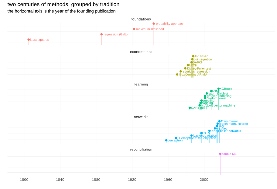

Figure 10.1: the methods of this book, placed in time

Two features of this picture deserve a comment. The econometric tradition is concentrated in twenty years, between the middle of the nineteen seventies and the end of the nineteen eighties, and it has been remarkably stable since: the tests of chapter seven are still the ones used today. The learning and network traditions, on the contrary, are spread out and accelerate, with a striking gap in the nineteen nineties for the networks, which is the second winter.