8.6 Pre-processing data

Almost everything in this chapter assumed that the matrix \(X\) was ready to use. It never is. This last section gathers the transformations that come before the model, and they deserve attention because they influence the result at least as much as the choice of the algorithm.

Scaling. Any method based on a distance or on a penalty is sensitive to the units, as we saw for the nearest neighbours, the support vector machine and the ridge regression. Two transformations are usual: standardization, which subtracts the mean and divides by the standard deviation, and min-max normalization, which maps the range onto \([0,1]\). Standardization is the default; min-max is used when a bounded interval is required, and it is far more sensitive to an extreme value. Trees and forests, which only compare thresholds within a single variable, need neither.

Categorical variables. A qualitative variable must be coded. One-hot coding creates one indicator per level, as the dummy variables of the chapter on multiple regression did. When a variable has very many levels this explodes the dimension, and other codings are used, for instance grouping the rare levels together.

Skewed variables. A variable with a long right tail, an income, a firm size, a price, is often replaced by its logarithm, which brings the distribution closer to symmetry and prevents a handful of large values from dominating a squared loss.

Unbalanced classes. When one class represents one per cent of the sample, the metrics of the earlier section must be chosen carefully, and the sample can also be rebalanced by drawing fewer majority observations, by duplicating minority ones, or by generating synthetic minority points with a method such as SMOTE. Any rebalancing must happen inside the training set alone.

The last point is the most important of the section, and it repeats the warning already given for imputation. Every transformation that learns something from the data, a mean, a standard deviation, a minimum, a set of levels, must learn it on the training set and then be applied unchanged to the test set. Otherwise information crosses from one to the other and the estimated performance becomes optimistic. The clean way of enforcing this is the pipeline, which chains the transformations and the model into a single object that can be fitted and cross validated as a whole.

In R:

set.seed(123)
inc <- rlnorm(500, meanlog = 10, sdlog = 1)     # a skewed variable

tr <- rbind(
  data.frame(value = inc, kind = "1. raw (skewed)"),
  data.frame(value = log(inc), kind = "2. logarithm"),
  data.frame(value = as.numeric(scale(inc)), kind = "3. standardized"),
  data.frame(value = (inc - min(inc)) / diff(range(inc)), kind = "4. min-max"))

ggplot(tr, aes(value)) +
  geom_histogram(bins = 40, fill = "steelblue", colour = "white") +
  facet_wrap(~ kind, nrow = 1, scales = "free") +
  labs(title = "a skewed variable under three transformations", x = "", y = "") +
  theme_minimal()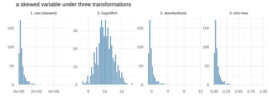

Figure 8.63: the effect of three transformations on the same variable

Standardizing and rescaling change the axis but not the shape: the asymmetry is still there, and a squared loss will still be dominated by the largest values. Only the logarithm changes the shape. This is worth remembering, because the two operations are often confused, and they solve different problems.

In Python:

The pipeline of scikit-learn is the cleanest way to guarantee that no transformation ever sees the test set.

from sklearn.compose import ColumnTransformer
from sklearn.linear_model import LogisticRegressionCV
from sklearn.preprocessing import StandardScaler, OneHotEncoder
from sklearn.impute import SimpleImputer
from sklearn.model_selection import cross_val_score

rng2 = np.random.default_rng(0)
m = 500
num1 = rng2.normal(size=m)
num2 = rng2.lognormal(mean=1.0, sigma=1.0, size=m)
cat = rng2.choice(["a", "b", "c"], size=m)
target = (0.9 * num1 + 0.4 * np.log(num2) + (cat == "a") * 0.8
          + rng2.normal(scale=0.5, size=m) > 0.7).astype(int)

dfp = pd.DataFrame({"num1": num1, "num2": num2, "cat": cat})
dfp.loc[rng2.choice(m, 60, replace=False), "num1"] = np.nan   # some holes

pre = ColumnTransformer([
    ("numeric", make_pipeline(SimpleImputer(strategy="median"), StandardScaler()),
     ["num1", "num2"]),
    ("categorical", OneHotEncoder(drop="first", handle_unknown="ignore"), ["cat"]),
])

pipe = make_pipeline(pre, LogisticRegressionCV(max_iter=2000))
scores = cross_val_score(pipe, dfp, target, cv=5, scoring="accuracy")

prep_py = pd.DataFrame({"fold": range(1, 6), "accuracy": np.round(scores, 4)})

Table 8.14: cross validated accuracy of the complete pipeline

fold	accuracy
1	0.76
2	0.84
3	0.86
4	0.84
5	0.83

The whole chain, imputation of the holes, standardization of the numeric variables, coding of the categorical one and estimation of the model, is contained in a single object. When the cross validation puts a fold aside, the imputer and the scaler are re-estimated on the remaining folds only, which is exactly the guarantee we wanted and which is very difficult to obtain by hand without a mistake.

This closes the chapter. We began by opposing the econometric question, what is the effect of \(x\) on \(y\), to the predictive one, how well can I predict \(y\) on data I have not seen, and everything that followed flowed from that second question: the separation between training and testing, the bias variance trade-off, the metrics, and a collection of algorithms each of which encodes a different assumption about the shape of the relation. The next chapter keeps the same objective and pushes the flexibility much further, by stacking layers of transformations that the model learns for itself.