7.5 Cointegration
We have insisted on the fact that a series with a unit root must be differenced before being used in a regression, because otherwise the classical results do not hold and the regression is spurious. This rule is safe, but it has a cost that economists are reluctant to accept: differencing destroys the information about the levels. If we regress the change of the consumption on the change of the income we learn something about the short run reaction, but we lose the long run relation between the two levels, which is often the very object of the economic theory we want to test.
Granger and Engle showed that this sacrifice is not always necessary. It may happen that two series are individually non stationary, each of them wandering without returning to any mean, and yet that a particular linear combination of the two is stationary. In that case the two series never drift far apart: they share a common stochastic trend, and the distance between them is a stationary process that always comes back towards its mean. We say that the two series are cointegrated, and the stationary combination is the long run relation.
Formally, two series integrated of order one, \(y_t\sim I(1)\) and \(x_t\sim I(1)\), are cointegrated if there exists a coefficient \(\beta\) such that:
\[\begin{equation} z_t=y_t-\beta x_t \sim I(0) \tag{7.45} \end{equation}\]
The vector \((1,-\beta)\) is the cointegrating vector, and \(z_t\) measures the deviation from the long run equilibrium at the date \(t\).
The strategy of Engle and Granger follows directly from this definition and proceeds in two steps:
estimate the long run relation \(y_t=\alpha+\beta x_t+z_t\) by ordinary least squares, on the levels;
apply a unit root test to the residuals \(\hat z_t\). If the unit root is rejected, the residuals are stationary and the two series are cointegrated.
The critical values of the second step are not those of Dickey and Fuller, because the residuals are not observed but estimated, which makes them artificially more stationary. The correct values, tabulated by Engle and Granger and by MacKinnon, are more negative.
To illustrate this, we build two series that share the same stochastic trend by construction.
In R:
set.seed(123)
n <- 400

# a common stochastic trend
common <- cumsum(rnorm(n))

# two I(1) series built on it
x_co <- common + rnorm(n, sd = 0.5)
y_co <- 2 + 1.5 * common + rnorm(n, sd = 0.5)

plot(y_co, type = "l", col = "black", ylab = "", main = "two cointegrated series")
lines(x_co, col = "red")
legend("topleft", legend = c("y", "x"), col = c("black", "red"), lty = 1, bty = "n")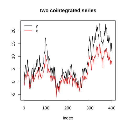
Figure 7.29: two cointegrated series
The two series wander, but they wander together. Neither of them returns to a fixed mean, and yet the vertical distance between them stays within a band.
# step 1: the long run relation, estimated on the levels
lr_fit <- lm(y_co ~ x_co)

# step 2: is the residual stationary ?
z_hat <- residuals(lr_fit)
eg_test <- ur.df(z_hat, type = "none", selectlags = "AIC")

eg_out <- data.frame(
  beta_long_run = coef(lr_fit)[2],
  adf_statistic = eg_test@teststat[1],
  crit_5pct     = eg_test@cval[1, "5pct"]
)| beta_long_run | adf_statistic | crit_5pct |
|---|---|---|
| 1.4724 | -14.6727 | -1.95 |
The estimated long run coefficient is close to the \(1.5\) that we used to build the series, and the statistic of the test on the residuals is far below the critical value, so the unit root is rejected: the residuals are stationary and the two series are cointegrated.
plot(z_hat, type = "l", ylab = "", main = "deviation from the long run equilibrium")
abline(h = 0, col = "red")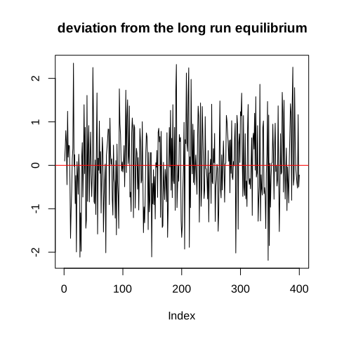
Figure 7.30: the residual of the long run relation
Contrary to the two original series, this one clearly oscillates around zero and crosses its mean regularly, which is the visual definition of a stationary process.
In Python:
The statsmodels package performs the two steps at once with the function coint, which returns the statistic, its p-value and the critical values.
from statsmodels.tsa.stattools import coint
import statsmodels.api as sm

stat, pval, crit = coint(y_co_py, x_co_py)

# the long run coefficient still comes from a regression on the levels
lr_py = sm.OLS(y_co_py, sm.add_constant(np.asarray(x_co_py))).fit()

coint_py = pd.DataFrame({
    "beta_long_run": [round(lr_py.params[1], 4)],
    "statistic": [round(stat, 4)],
    "p_value": [round(pval, 4)],
    "crit_5pct": [round(crit[1], 4)]
})| beta_long_run | statistic | p_value | crit_5pct |
|---|---|---|---|
| 1.4724 | -19.744 | 0 | -3.3515 |
The p-value is very small, so the null hypothesis of absence of cointegration is rejected, and the conclusion is the same as in R.
The Engle-Granger procedure has two limitations that should be kept in mind. It can only find one cointegrating relation, whereas a system of \(g\) variables may contain up to \(g-1\) of them, and the result may depend on which variable is placed on the left hand side of the first regression. The Johansen methodology, presented at the end of this chapter, answers both objections by working on the whole system at once.
7.5.1 The error correction model ECM
Cointegration tells us that a long run relation exists, but it says nothing about the speed at which the variables come back to it after a shock. The error correction model answers this second question, and it is the natural companion of the previous section.
The representation theorem of Granger states that two series are cointegrated if and only if they admit an error correction representation. For two variables this representation is written:
\[\begin{equation} \vartriangle y_t=\mu+\gamma\vartriangle x_t+\lambda \hat z_{t-1}+\varepsilon_t \tag{7.46} \end{equation}\]
where \(\hat z_{t-1}=y_{t-1}-\hat\alpha-\hat\beta x_{t-1}\) is the deviation from the long run equilibrium observed at the previous period. The equation contains therefore two very different pieces of information:
the coefficient \(\gamma\) describes the short run effect, the immediate reaction of \(y\) to a change of \(x\);
the coefficient \(\lambda\) describes the adjustment, the fraction of the past disequilibrium that is corrected during the current period.
The sign of \(\lambda\) must be negative for the mechanism to make sense: if \(y\) was above its long run value at \(t-1\), then \(\hat z_{t-1}>0\), and the term \(\lambda \hat z_{t-1}\) pulls \(\vartriangle y_t\) downwards, bringing the series back towards the equilibrium. A value of \(\lambda=-0.3\) means that thirty per cent of the gap is closed every period, and that the half-life of a shock is a little more than two periods. A coefficient that is not significant, or positive, indicates that the error correction mechanism does not exist, which contradicts the cointegration found in the first step.
This model also solves the dilemma we started from: all the terms of the equation are stationary, since \(\vartriangle y_t\) and \(\vartriangle x_t\) are differences of \(I(1)\) series and \(\hat z_{t-1}\) is stationary by construction, so the classical inference is valid again. And yet the long run information has not been lost, it is carried by the error correction term.
In R:
# the deviation from the equilibrium, lagged by one period
z_lag <- z_hat[-length(z_hat)]
dy    <- diff(y_co)
dx    <- diff(x_co)

ecm_fit <- lm(dy ~ dx + z_lag)

ecm_out <- data.frame(
  coefficient = c("intercept", "short run (dx)", "adjustment (z_lag)"),
  estimate    = as.numeric(coef(ecm_fit)),
  std_error   = as.numeric(summary(ecm_fit)$coefficients[, 2]),
  p_value     = as.numeric(summary(ecm_fit)$coefficients[, 4])
)| coefficient | estimate | std_error | p_value |
|---|---|---|---|
| intercept | 0.0058 | 0.0414 | 0.8891 |
| short run (dx) | 1.1529 | 0.0364 | 0.0000 |
| adjustment (z_lag) | -0.8308 | 0.0494 | 0.0000 |
The adjustment coefficient is negative and strongly significant, as the theory requires. Its magnitude tells us how quickly the system absorbs a disequilibrium.
In Python:
z_hat_py = np.asarray(lr_py.resid)
dy_py = np.diff(np.asarray(y_co_py))
dx_py = np.diff(np.asarray(x_co_py))
z_lag_py = z_hat_py[:-1]

X_ecm = sm.add_constant(np.column_stack([dx_py, z_lag_py]))
ecm_py = sm.OLS(dy_py, X_ecm).fit()

ecm_out_py = pd.DataFrame({
    "coefficient": ["intercept", "short run (dx)", "adjustment (z_lag)"],
    "estimate": [round(v, 4) for v in ecm_py.params],
    "std_error": [round(v, 4) for v in ecm_py.bse],
    "p_value": [round(v, 4) for v in ecm_py.pvalues]
})| coefficient | estimate | std_error | p_value |
|---|---|---|---|
| intercept | 0.0058 | 0.0414 | 0.8891 |
| short run (dx) | 1.1529 | 0.0364 | 0.0000 |
| adjustment (z_lag) | -0.8308 | 0.0494 | 0.0000 |