9.4 Regularization
A network with a few hundred thousand parameters can memorize a training set of a few thousand observations, and it will do so if nothing prevents it. Everything in this section exists to prevent it.
The problem is the same bias variance trade-off as in the previous chapter, but it takes a particular form here. In a classical model we controlled the complexity by choosing the number of variables or the degree of a polynomial. In a network we usually want a large capacity, because it makes the optimization easier, and we then restrain it by other means. The modern practice is therefore to take a model that is too big and to regularize it, rather than to look for the model of exactly the right size.
9.4.1 Overfitting in a network
Let us first see the phenomenon. We take a small sample, a network large enough to memorize it, and we follow the two losses.
In R:
set.seed(123)

# a small training set and a large validation set from the same law
n_tr <- 60
Xtr <- matrix(rnorm(n_tr * 2), n_tr, 2)
ytr <- as.numeric(Xtr[, 1]^2 + Xtr[, 2]^2 > 1.6)
Xva <- matrix(rnorm(600 * 2), 600, 2)
yva <- as.numeric(Xva[, 1]^2 + Xva[, 2]^2 > 1.6)

train_track <- function(h = 60, eta = .35, steps = 3000, lambda = 0) {
  net <- init_net(2, h, seed = 7)
  tr <- va <- numeric(steps)
  for (s in 1:steps) {
    fw <- forward(net, Xtr)
    g  <- backward(net, Xtr, ytr, fw)
    # weight decay: the derivative of (lambda/2)*sum(W^2) is lambda*W
    net$W1 <- net$W1 - eta * (g$W1 + lambda * net$W1); net$b1 <- net$b1 - eta * g$b1
    net$W2 <- net$W2 - eta * (g$W2 + lambda * net$W2); net$b2 <- net$b2 - eta * g$b2
    tr[s] <- loss_fn(fw$yhat, ytr)
    va[s] <- loss_fn(forward(net, Xva)$yhat, yva)
  }
  list(net = net, df = rbind(
    data.frame(step = 1:steps, loss = tr, set = "training"),
    data.frame(step = 1:steps, loss = va, set = "validation")))
}

plain <- train_track()

ggplot(plain$df, aes(step, loss, colour = set)) +
  geom_line(linewidth = .8) +
  geom_vline(xintercept = which.min(plain$df$loss[plain$df$set == "validation"]),
             linetype = 2, colour = "grey40") +
  labs(title = "a network with 60 hidden units on 60 observations",
       subtitle = "the dashed line marks the minimum of the validation loss") +
  theme_minimal()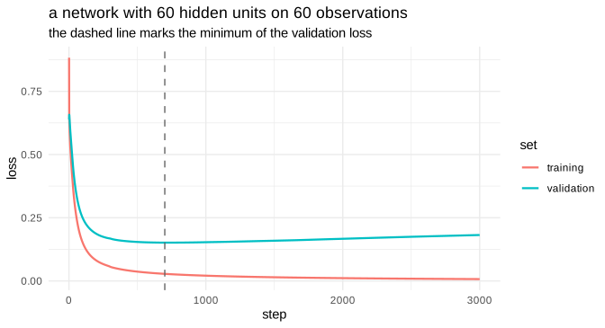
Figure 9.15: the two losses separate as soon as the network starts memorizing
The training loss decreases without limit, since the network has enough parameters to pass through every point. The validation loss decreases, reaches a minimum, and then rises: from that point on, everything the network learns is particular to the training sample. The dashed line is the moment at which training should have stopped, and it is the subject of one of the sections below.
9.4.2 Weight decay
The first remedy is the one we already know from the ridge and the lasso: add a penalty on the size of the weights.
\[\begin{equation} L_{total}=L_{data}+\frac{\lambda}{2}\sum_{l}\lVert W^{(l)}\rVert^2 \tag{9.17} \end{equation}\]
Its gradient is \(\lambda W\), so the update becomes \(W \leftarrow W-\eta(\nabla L_{data}+\lambda W)\), which shrinks every weight by a constant factor at each step. This is why it is called weight decay in this literature; it is exactly the ridge penalty of the previous chapter.
The \(L_2\) penalty is by far the most common. The \(L_1\) penalty is used when a sparse network is wanted, since it sets weights exactly to zero, but pruning a trained network usually works better in practice.
Two practical points. The biases are not penalized: they only shift the activation and do not control the complexity. And the penalty interacts with the optimizer, which is why the variant AdamW separates the decay from the adaptive rescaling instead of adding it to the gradient.
In R:
pen <- train_track(lambda = 0.02)

w_df <- rbind(
  data.frame(w = as.numeric(plain$net$W1), kind = "without penalty"),
  data.frame(w = as.numeric(pen$net$W1),   kind = "with penalty"))

wd1 <- ggplot(w_df, aes(w, fill = kind)) +
  geom_histogram(bins = 40, alpha = .6, position = "identity") +
  labs(title = "distribution of the weights of the first layer") +
  theme_minimal() + theme(legend.position = "bottom")

both <- rbind(cbind(plain$df, model = "without penalty"),
              cbind(pen$df,   model = "with penalty"))

wd2 <- ggplot(subset(both, set == "validation"),
              aes(step, loss, colour = model)) +
  geom_line(linewidth = .8) +
  labs(title = "validation loss") +
  theme_minimal() + theme(legend.position = "bottom")

wd1 + wd2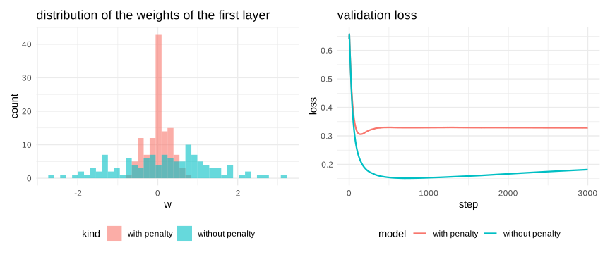
Figure 9.16: the effect of the penalty on the weights and on the boundary
The penalized weights are visibly concentrated around zero, and the validation loss no longer rises in the same way: the network is prevented from building the very large weights that a sharp, memorizing boundary requires.
9.4.3 Dropout
Dropout is a specifically neural idea, and a strange one at first sight. At each training step, every neuron of a layer is removed with probability \(p\), together with all its connections. The network that performs the update is therefore a different, thinner network at every iteration.
Two ways of understanding why this helps. First, a neuron can no longer rely on the presence of a particular colleague, since that colleague may disappear at any moment; it must therefore contribute something useful on its own, which prevents the fragile co-adaptations that memorization relies on. Second, training with dropout amounts to training an enormous ensemble of thinned networks that share their weights, and we know from the previous chapter that averaging models reduces the variance.
At test time nothing is dropped, because we want a deterministic prediction. The activations are then scaled so that their expectation matches the one seen during training; in practice the scaling is applied during training instead, dividing by \(1-p\), which is called inverted dropout and leaves the test path untouched.
Typical values are \(p=0.5\) for the dense layers and \(p=0.1\) to \(0.3\) for the convolutional ones, which have far fewer parameters and need less of it.
In R:
set.seed(2)
lay <- expand.grid(unit = 1:10, step = 1:6)
lay$kept <- runif(nrow(lay)) > 0.4

ggplot(lay, aes(step, unit, fill = kept)) +
  geom_tile(colour = "white", linewidth = 1) +
  scale_fill_manual(values = c("grey85", "steelblue")) +
  labs(title = "a layer of ten units over six training steps",
       subtitle = "grey = temporarily removed", x = "training step", y = "unit") +
  theme_minimal() + theme(legend.position = "none")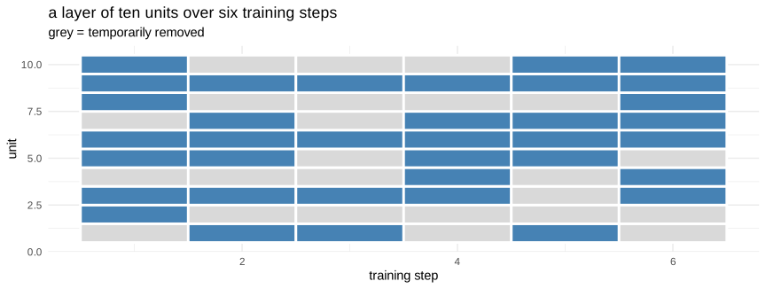
Figure 9.17: dropout switches off a different subset at every step
train_drop <- function(h = 60, eta = .35, steps = 3000, p_drop = .5) {
  net <- init_net(2, h, seed = 7)
  tr <- va <- numeric(steps)
  for (s in 1:steps) {
    Z1 <- Xtr %*% t(net$W1) + matrix(net$b1, nrow(Xtr), h, byrow = TRUE)
    A1 <- relu(Z1)
    mask <- matrix(rbinom(length(A1), 1, 1 - p_drop), nrow(A1), ncol(A1))
    A1d <- A1 * mask / (1 - p_drop)            # inverted dropout
    Z2 <- as.numeric(A1d %*% t(net$W2) + net$b2)
    yh <- sigm(Z2)

    m <- nrow(Xtr)
    d2 <- (yh - ytr) / m
    gW2 <- matrix(d2 %*% A1d, 1, h); gb2 <- sum(d2)
    d1 <- outer(d2, as.numeric(net$W2)) * (mask / (1 - p_drop)) * drelu(Z1)
    gW1 <- t(d1) %*% Xtr; gb1 <- colSums(d1)

    net$W1 <- net$W1 - eta * gW1; net$b1 <- net$b1 - eta * gb1
    net$W2 <- net$W2 - eta * gW2; net$b2 <- net$b2 - eta * gb2

    tr[s] <- loss_fn(forward(net, Xtr)$yhat, ytr)   # no dropout at evaluation
    va[s] <- loss_fn(forward(net, Xva)$yhat, yva)
  }
  rbind(data.frame(step = 1:steps, loss = tr, set = "training"),
        data.frame(step = 1:steps, loss = va, set = "validation"))
}

dr <- train_drop()

comp_dr <- rbind(cbind(subset(plain$df, set == "validation"), model = "no dropout"),
                 cbind(subset(dr,       set == "validation"), model = "dropout 0.5"))

ggplot(comp_dr, aes(step, loss, colour = model)) +
  geom_line(linewidth = .8) +
  labs(title = "validation loss with and without dropout") +
  theme_minimal()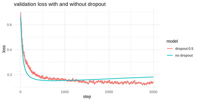
Figure 9.18: dropout on the same overfitting problem
Note in the code that the mask must be applied in the backward pass as well: a unit that was switched off contributed nothing to the output and must receive no gradient. Forgetting this is a classical bug, and it produces a network that trains slowly for no visible reason.
9.4.4 Early stopping
The first figure of this section already showed the principle. The validation loss has a minimum; we monitor it during training and we keep the parameters of the moment when it was lowest, rather than those of the last epoch.
Two parameters govern it in practice. The patience is the number of epochs we accept to continue without improvement before stopping, because the curve is noisy and a single bad epoch means nothing. And the weights of the best epoch must actually be saved, otherwise we stop at a point that is already worse than the best one seen.
Early stopping is the cheapest regularizer of all, since it costs nothing but the validation set, and for that reason it is used almost systematically, in combination with the others rather than instead of them.
In R:
va_curve <- subset(plain$df, set == "validation")
best <- which.min(va_curve$loss)
patience <- 400
stop_at <- min(best + patience, nrow(va_curve))

ggplot(va_curve, aes(step, loss)) +
  geom_line(colour = "steelblue", linewidth = .8) +
  geom_vline(xintercept = best, colour = "firebrick", linetype = 2) +
  geom_vline(xintercept = stop_at, colour = "grey40", linetype = 3) +
  # ggplot2:: is required here: the tm package, loaded by the topic model of
  # the previous chapter, exports its own annotate() and masks this one.
  ggplot2::annotate("text", x = best, y = max(va_curve$loss) * .95,
           label = "best epoch, weights kept", hjust = -0.05, size = 3) +
  ggplot2::annotate("text", x = stop_at, y = max(va_curve$loss) * .85,
           label = "training actually stops here", hjust = -0.05, size = 3) +
  labs(title = "the patience lets the curve be noisy") +
  theme_minimal()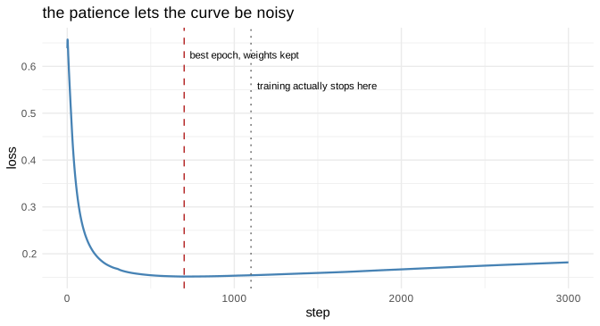
Figure 9.19: early stopping keeps the parameters of the best epoch
9.4.5 Batch normalization
Batch normalization attacks a different problem: the distribution of the inputs of a layer keeps changing during training, because the layers below are themselves changing. Each layer must therefore constantly re-adapt to a moving target, which slows everything down.
The remedy is to normalize the pre-activations inside each mini-batch:
\[\begin{equation} \hat z=\frac{z-\mu_{batch}}{\sqrt{\sigma^2_{batch}+\epsilon}}, \qquad y=\gamma\hat z+\beta \tag{9.18} \end{equation}\]
The first part centres and scales, the second restores the freedom that the first removed, through two parameters \(\gamma\) and \(\beta\) that are learned like any other. The network can therefore undo the normalization if that is useful, but it starts from a well conditioned state.
The effects are large and partly still debated. Training becomes much less sensitive to the initialization and tolerates larger learning rates; and the statistics of a batch depend on the other observations in it, which injects noise and acts as a mild regularizer. This last property is why batch normalization and dropout are often not both needed.
One point requires attention: at test time there is no batch, so the running averages of \(\mu\) and \(\sigma^2\) accumulated during training are used instead. A network in training mode and the same network in evaluation mode therefore do not compute the same thing, and forgetting to switch modes is one of the most common errors in practice.
In R:
set.seed(1)
depth <- 10; width <- 128

propagate <- function(use_bn) {
  A <- matrix(rnorm(width), 1, width)
  out <- data.frame()
  for (l in 1:depth) {
    W <- matrix(rnorm(width * width, sd = .12), width, width)  # deliberately bad scale
    Z <- A %*% W
    if (use_bn) Z <- (Z - mean(Z)) / (sd(Z) + 1e-8)
    A <- pmax(Z, 0)
    out <- rbind(out, data.frame(layer = l, sd = sd(as.numeric(Z)),
                                 kind = if (use_bn) "with batch norm" else "without"))
  }
  out
}

bn <- rbind(propagate(FALSE), propagate(TRUE))

ggplot(bn, aes(layer, sd, colour = kind)) +
  geom_line(linewidth = .9) + geom_point() +
  scale_y_log10() +
  labs(title = "standard deviation of the pre-activations, layer by layer",
       y = "sd (log scale)") +
  theme_minimal()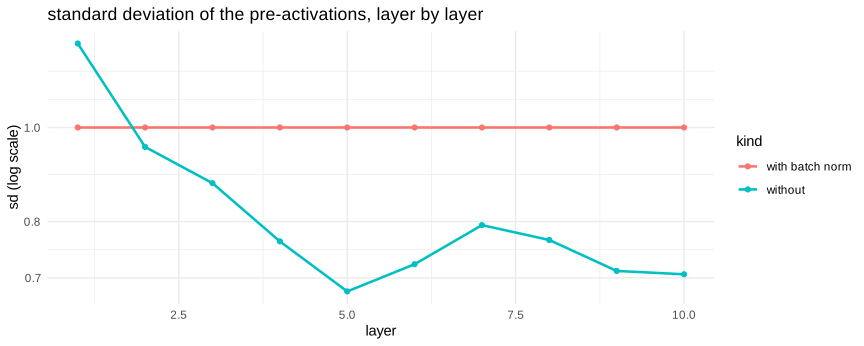
Figure 9.20: the distribution of the pre-activations across a deep network
Without normalization and with a poorly chosen scale, the signal collapses layer after layer, which is the vanishing problem of the previous section seen on the forward pass. With batch normalization it stays at the same level whatever the depth, and this is the practical reason for its success.
9.4.6 Data augmentation
The last regularizer does not touch the model at all: it enlarges the data. If we know a transformation that changes the input without changing the label, we can apply it at random during training and obtain, in effect, a much larger sample.
For images the transformations are geometric and photometric: small rotations, translations, changes of scale, horizontal flips, changes of brightness and contrast, random crops. For a time series one may add noise, shift the window or rescale the amplitude. For text, replacing words by synonyms or back-translating through another language.
The condition is written in the definition and it is easy to violate: the transformation must preserve the label. Flipping a photograph of a cat horizontally still shows a cat; flipping the digit \(2\) horizontally does not give a \(2\), and a network trained on such images learns something false. Augmentation always encodes an assumption about the invariances of the problem, and that assumption must be true.
In Python:
We use the small handwritten digits bundled with scikit-learn, eight by eight pixels, which need no download and will serve again in the next section.
from sklearn.datasets import load_digits
from scipy.ndimage import rotate, shift, zoom

digits = load_digits()
img = digits.images[17]

def augment(im, rng):
    out = rotate(im, rng.uniform(-12, 12), reshape=False, order=1, mode="nearest")
    out = shift(out, (rng.uniform(-1, 1), rng.uniform(-1, 1)), order=1, mode="nearest")
    out = out * rng.uniform(0.8, 1.2)
    return np.clip(out, 0, 16)

rng_aug = np.random.default_rng(0)
fig, axes = plt.subplots(1, 7, figsize=(10, 1.8))
axes[0].imshow(img, cmap="gray_r"); axes[0].set_title("original", fontsize=8)
#> <matplotlib.image.AxesImage object at 0x0000020F2C690560>
#> Text(0.5, 1.0, 'original')for ax in axes[1:]:
ax.imshow(augment(img, rng_aug), cmap="gray_r")
ax.set_title("augmented", fontsize=8)#> <matplotlib.image.AxesImage object at 0x0000020F2C6FE030>
#> Text(0.5, 1.0, 'augmented')
#> <matplotlib.image.AxesImage object at 0x0000020F2C71C260>
#> Text(0.5, 1.0, 'augmented')
#> <matplotlib.image.AxesImage object at 0x0000020F2C7B5400>
#> Text(0.5, 1.0, 'augmented')
#> <matplotlib.image.AxesImage object at 0x0000020F2C755940>
#> Text(0.5, 1.0, 'augmented')
#> <matplotlib.image.AxesImage object at 0x0000020F2C781B20>
#> Text(0.5, 1.0, 'augmented')
#> <matplotlib.image.AxesImage object at 0x0000020F2C7B6660>
#> Text(0.5, 1.0, 'augmented')#> []
#> []
#> []
#> []
#> []
#> []
#> []
#> []
#> []
#> []
#> []
#> []
#> []
#> []
Figure 9.21: data augmentation on a handwritten digit
Every image on the right is still recognizably the same digit, which is the condition we stated, and each of them is a new training example that the network has never seen. On small image data sets this technique alone often improves the accuracy more than any change of architecture.
The augmentation is applied to the training set only. Augmenting the validation or the test set changes the problem on which the model is judged and makes the comparison meaningless, exactly as imputing or scaling on the whole data did in the previous chapter.