7.3 ARIMA models

The processes described at the beginning of this chapter were theoretical objects. We knew the orders and the coefficients because we had chosen them ourselves. With real data nothing of that is given, and the whole work consists in recovering them from a single realization of the process. The methodology that organizes this work is due to Box and Jenkins, and it proceeds in four steps that we follow in the sections below:

Identification: we make the series stationary if it is not, using the unit root tests of the previous section, and we read the correlogram and the partial correlogram to propose a small number of candidate orders.
Estimation: we estimate the coefficients of each candidate model.
Diagnostic checking: we verify that the residuals of the retained model behave as a white noise. If they do not, the model has missed a part of the dynamic and we go back to the first step.
Forecasting: once the model is validated, we use it to predict the future values of the series.

The general model that gathers the three components is the \(ARIMA(p,d,q)\), where \(p\) is the auto-regressive order, \(d\) the number of differences needed to remove the unit roots, and \(q\) the moving average order. Written with the lag operator it takes the compact form:

\[\begin{equation} \Phi(D)(1-D)^dy_t=\Theta(D)\varepsilon_t \tag{7.32} \end{equation}\]

where \(\Phi(D)=1-\phi_1D-...-\phi_pD^p\) and \(\Theta(D)=1+\theta_1D+...+\theta_qD^q\). Each of the models of this section is a particular case of this equation.

7.3.1 AR model

The auto-regressive process was defined in equation (7.8). Estimating it is comparatively easy, because the regressors are the lagged values of the series and they are observed. Three methods are commonly used:

the Yule-Walker equations, which express the coefficients as a function of the autocorrelations and solve a linear system;
the ordinary least squares, applied to the regression of \(y_t\) on its \(p\) lags, which is consistent although slightly biased in small samples;
the maximum likelihood, which assumes normal errors and is the method used by default by most software.

Let us simulate an \(AR(2)\) with known coefficients and see whether the estimation recovers them.

In R:

set.seed(123)

# simulate an AR(2) with phi1 = 0.6 and phi2 = -0.3
ar2_ts <- arima.sim(model = list(ar = c(0.6, -0.3)), n = 400)

par(mfrow = c(1, 2))
Acf(ar2_ts, main = "ACF")
Pacf(ar2_ts, main = "PACF")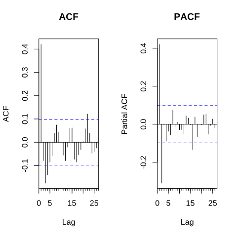

Figure 7.16: correlogram and partial correlogram of an AR(2)

par(mfrow = c(1, 1))

The partial correlogram shows two spikes and then nothing, which points to an \(AR(2)\), while the correlogram decays. This is the mirror rule of the previous section, and it gives us the candidate order without knowing the answer in advance.

# estimation by maximum likelihood
ar2_fit <- arima(ar2_ts, order = c(2, 0, 0))

ar2_out <- data.frame(
  coefficient = names(ar2_fit$coef),
  true_value  = c(0.6, -0.3, 0),
  estimate    = as.numeric(ar2_fit$coef),
  std_error   = sqrt(diag(ar2_fit$var.coef))
)

Table 7.7: estimation of an AR(2) in R
	coefficient	true_value	estimate	std_error
ar1	ar1	0.6	0.550	0.0475
ar2	ar2	-0.3	-0.309	0.0475
intercept	intercept	0.0	0.009	0.0634

The two estimates are close to the values used in the simulation, and the intercept is not significantly different from zero, which is expected since we simulated the process without a constant.

In Python:

The statsmodels package estimates the same model through the class ARIMA, giving the order \((p,d,q)=(2,0,0)\).

if 'ar2_py' not in globals():
  ar2_py = r.ar2_ts


from statsmodels.tsa.arima.model import ARIMA

ar2_fit_py = ARIMA(ar2_py, order=(2, 0, 0)).fit()
ar2_out_py = pd.DataFrame({
    "coefficient": ar2_fit_py.params.index.astype(str) if hasattr(ar2_fit_py.params, "index") else ["const", "ar.L1", "ar.L2", "sigma2"],
    "estimate": [round(v, 4) for v in ar2_fit_py.params],
    "std_error": [round(v, 4) for v in ar2_fit_py.bse]
})

Table 7.8: estimation of an AR(2) in python
coefficient	estimate	std_error
const	0.0090	0.0644
ar.L1	0.5500	0.0458
ar.L2	-0.3090	0.0492
sigma2	0.9254	0.0694

The coefficients agree with those obtained in R. The small differences come from the optimizer and from the way each package treats the first observations, not from the model itself.

Before using a model we must check its residuals. If the model has captured the whole dynamic, what remains should be a white noise, with no significant spike in the correlogram. The Ljung-Box test formalizes this idea by testing jointly that the first \(h\) autocorrelations of the residuals are null:

\[\begin{equation} Q=n(n+2)\sum_{k=1}^{h}\frac{\hat\gamma_k^2}{n-k} \tag{7.33} \end{equation}\]

Under the null hypothesis of no autocorrelation, \(Q\) follows a \(\chi^2\) distribution. A large p-value is therefore good news for the model.

# diagnostic on the residuals
box_ar2 <- Box.test(residuals(ar2_fit), lag = 10, type = "Ljung-Box", fitdf = 2)
box_ar2

#> 
#>  Box-Ljung test
#> 
#> data:  residuals(ar2_fit)
#> X-squared = 7.1247, df = 8, p-value = 0.5232

The p-value is large, so we do not reject the hypothesis that the residuals are a white noise, and the \(AR(2)\) is validated.

7.3.2 Impulse response function IRF

The coefficients of an auto-regressive model are not easy to read directly, because a change in \(y_{t-1}\) propagates to \(y_t\), then to \(y_{t+1}\), and so on. The impulse response function answers a simpler question: if the process receives a single shock of one unit at the date \(t\), and no shock afterwards, what happens to the series in the following periods?

The answer comes from the moving average representation of the process. We have shown for the \(AR(1)\) that it can be written as an infinite sum of past shocks, and the general \(ARMA\) admits the same \(MA(\infty)\) form:

\[\begin{equation} y_t=\sum_{k=0}^{\infty}\psi_k\varepsilon_{t-k} \quad \text{with} \quad \psi_0=1 \tag{7.34} \end{equation}\]

The coefficient \(\psi_k\) is precisely the effect, after \(k\) periods, of a unit shock received today. The sequence \(\{\psi_k\}\) is the impulse response function. For an \(AR(1)\) we already know it, since \(y_t=\varepsilon_t+\phi\varepsilon_{t-1}+\phi^2\varepsilon_{t-2}+...\), hence:

\[\begin{equation} \psi_k=\phi^k \tag{7.35} \end{equation}\]

The shock therefore fades geometrically when \(\lvert\phi\rvert<1\), and the speed of the decay measures the persistence of the process. In the unit root case \(\phi=1\) we get \(\psi_k=1\) for every \(k\), which is the formal translation of what we said earlier: the shock never dies out.

In R:

The function ARMAtoMA converts the auto-regressive and moving average coefficients into the \(\psi_k\) weights.

# psi weights of the estimated AR(2)
psi <- ARMAtoMA(ar = ar2_fit$coef[c("ar1", "ar2")], ma = 0, lag.max = 20)
psi <- c(1, psi)

plot(0:20, psi, type = "h", lwd = 2,
     xlab = "periods after the shock", ylab = "response",
     main = "Impulse response of the AR(2)")
abline(h = 0)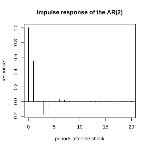

Figure 7.17: impulse response function of the estimated AR(2)

The response is positive at the first period, becomes negative afterwards because \(\phi_2\) is negative, and converges towards zero. The oscillation is the signature of an auto-regressive process of order two with a negative second coefficient.

In Python:

The class ArmaProcess of statsmodels provides the same weights through its method impulse_response.

import numpy as np
import matplotlib.pyplot as plt
from statsmodels.tsa.arima_process import ArmaProcess

phi = [ar2_fit_py.params[1], ar2_fit_py.params[2]]
proc = ArmaProcess(np.r_[1, -np.array(phi)], np.array([1]))
irf = proc.impulse_response(21)

plt.figure(figsize=(5, 3))

#> <Figure size 500x300 with 0 Axes>

plt.stem(range(21), irf)

#> <StemContainer object of 3 artists>

plt.axhline(0, color="black", linewidth=0.8)

#> <matplotlib.lines.Line2D object at 0x0000020E9CCE10A0>

plt.xlabel("periods after the shock")

#> Text(0.5, 0, 'periods after the shock')

plt.ylabel("response")

#> Text(0, 0.5, 'response')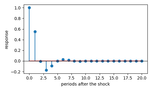

plt.tight_layout()
plt.savefig("irf_py.png")
plt.clf()
plt.close()

Figure 7.18: impulse response function in python

Note that the sign convention of the auto-regressive polynomial is not the same in the two packages. R stores the \(\phi_i\) as they appear in equation (7.8), while ArmaProcess expects the coefficients of the polynomial \(\Phi(D)\), that is \(1-\phi_1D-\phi_2D^2\). This is the reason for the sign change in the code above, and forgetting it is a frequent source of confusion.

7.3.3 MA model

The moving average process of equation defined earlier expresses the series as a combination of past shocks. Its estimation raises a difficulty that the auto-regressive case did not have: the regressors \(\varepsilon_{t-1},...,\varepsilon_{t-q}\) are not observed. The ordinary least squares are therefore impossible to apply directly, and we must rely on the maximum likelihood, which reconstructs the shocks recursively from an initial value and maximizes the likelihood of the observed series.

An \(MA(q)\) is also required to be invertible, that is to admit an \(AR(\infty)\) representation, which happens when the roots of \(\Theta(D)=0\) lie outside the unit circle. Without this condition several sets of coefficients would give exactly the same autocorrelations, and the model would not be identified.

In R:

set.seed(123)

# simulate an MA(1) with theta = 0.7
ma1_ts <- arima.sim(model = list(ma = 0.7), n = 400)

par(mfrow = c(1, 2))
Acf(ma1_ts, main = "ACF")
Pacf(ma1_ts, main = "PACF")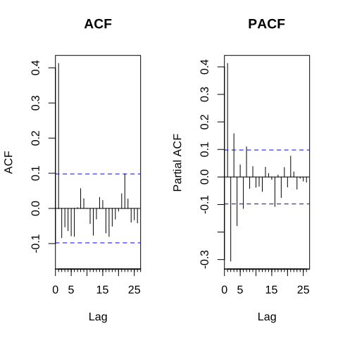

Figure 7.19: correlogram and partial correlogram of an MA(1)

par(mfrow = c(1, 1))

This time the correlogram has a single spike and the partial correlogram decays, which is the opposite configuration of the \(AR(2)\) and points to an \(MA(1)\).

ma1_fit <- arima(ma1_ts, order = c(0, 0, 1))

ma1_out <- data.frame(
  coefficient = names(ma1_fit$coef),
  true_value  = c(0.7, 0),
  estimate    = as.numeric(ma1_fit$coef),
  std_error   = sqrt(diag(ma1_fit$var.coef))
)

Table 7.9: estimation of an MA(1) in R
	coefficient	true_value	estimate	std_error
ma1	ma1	0.7	0.7288	0.0407
intercept	intercept	0.0	0.0276	0.0835

In Python:

if 'ma1_py' not in globals():
  ma1_py = r.ma1_ts


ma1_fit_py = ARIMA(ma1_py, order=(0, 0, 1)).fit()
ma1_out_py = pd.DataFrame({
    "coefficient": ["const", "ma.L1", "sigma2"],
    "estimate": [round(v, 4) for v in ma1_fit_py.params],
    "std_error": [round(v, 4) for v in ma1_fit_py.bse]
})

Table 7.10: estimation of an MA(1) in python
coefficient	estimate	std_error
const	0.0276	0.0847
ma.L1	0.7288	0.0356
sigma2	0.9353	0.0685

Both packages recover a coefficient close to the \(0.7\) used in the simulation.

7.3.4 ARMA model

Nothing prevents a series from carrying at the same time an auto-regressive and a moving average component. The \(ARMA(p,q)\) model gathers the two:

\[\begin{equation} y_t=\phi_1y_{t-1}+...+\phi_py_{t-p}+\varepsilon_t+\theta_1\varepsilon_{t-1}+...+\theta_q\varepsilon_{t-q} \tag{7.36} \end{equation}\]

The interest of this combination is parsimony. A pure auto-regressive model may need a large number of lags to reproduce a dynamic that an \(ARMA(1,1)\) describes with two coefficients, and every additional coefficient is estimated with an error that degrades the forecasts.

The counterpart is that the identification becomes harder. When both components are present, neither the correlogram nor the partial correlogram cuts off cleanly, and the mirror rule no longer gives an obvious answer. We therefore estimate several candidate models and compare them with an information criterion, which balances the fit against the number of coefficients:

\[\begin{align} &AIC=-2\ln(L)+2k \\ &BIC=-2\ln(L)+k\ln(n) \end{align}\]

where \(L\) is the likelihood, \(k\) the number of estimated parameters and \(n\) the number of observations. The \(BIC\) penalizes the complexity more heavily than the \(AIC\), and therefore tends to select smaller models.

In R:

set.seed(123)

# simulate an ARMA(1,1)
arma_ts <- arima.sim(model = list(ar = 0.6, ma = 0.4), n = 400)

# compare all the models up to order 2 with the AIC and the BIC
grid <- expand.grid(p = 0:2, q = 0:2)
grid$aic <- NA
grid$bic <- NA
for (i in seq_len(nrow(grid))) {
  fit <- try(arima(arma_ts, order = c(grid$p[i], 0, grid$q[i])), silent = TRUE)
  if (!inherits(fit, "try-error")) {
    grid$aic[i] <- AIC(fit)
    grid$bic[i] <- BIC(fit)
  }
}
grid <- grid[order(grid$aic), ]

Table 7.11: selection of the orders of an ARMA in R
p	q	aic	bic
1	1	1110.30	1126.27
2	1	1111.94	1131.90
1	2	1112.12	1132.08
2	2	1113.71	1137.66
2	0	1116.97	1132.93

The smallest \(AIC\) is obtained for the orders that we used in the simulation, which confirms that the criterion does its job here. On real data the answer is rarely so clean, and it is wise to look at the first few models of the table rather than at the very first one only.

The R package forecast automates this search with the function auto.arima, which explores the orders and returns the best model according to the chosen criterion.

auto_fit <- auto.arima(arma_ts, seasonal = FALSE, stepwise = FALSE, approximation = FALSE)
auto_fit

#> Series: arma_ts 
#> ARIMA(3,0,1) with zero mean 
#> 
#> Coefficients:
#>          ar1     ar2      ar3     ma1
#>       0.0708  0.4247  -0.1638  0.8838
#> s.e.  0.0840  0.0863   0.0615  0.0647
#> 
#> sigma^2 = 0.9187:  log likelihood = -549.11
#> AIC=1108.23   AICc=1108.38   BIC=1128.18

The function explores orders beyond the ones of our small grid, and it returns here an \(ARIMA(3,0,1)\) whose \(AIC\) is very slightly lower than the one of the \(ARMA(1,1)\). This is a good illustration of the limits of the exercise: the \(AIC\) rewards the fit, and with four coefficients instead of two it is almost always possible to gain a fraction of a point. The \(BIC\), which penalizes the complexity more heavily, keeps the \(ARMA(1,1)\), and so does the principle of parsimony. When two models are so close, the simpler one should be preferred, especially if the goal is to forecast.

In Python:

There is no direct equivalent of auto.arima in statsmodels, so we write the same loop ourselves.

if 'arma_py' not in globals():
  arma_py = r.arma_ts


import itertools
import warnings
warnings.filterwarnings("ignore")

rows = []
for p, q in itertools.product(range(3), range(3)):
    try:
        res = ARIMA(arma_py, order=(p, 0, q)).fit()
        rows.append({"p": p, "q": q, "aic": round(res.aic, 2), "bic": round(res.bic, 2)})
    except Exception:
        pass

grid_py = pd.DataFrame(rows).sort_values("aic").head(5).reset_index(drop=True)

Table 7.12: selection of the orders of an ARMA in python
p	q	aic	bic
1	1	1110.30	1126.27
2	2	1111.52	1135.47
2	1	1111.94	1131.90
1	2	1112.12	1132.08
2	0	1116.97	1132.93

The best model is the same as the one obtained in R, with the same value of the criterion.

7.3.5 Integrated ARMA model ARIMA

The models above all require a stationary series. When the unit root tests conclude that the series is not stationary, we difference it \(d\) times until it becomes so, and we fit an \(ARMA(p,q)\) to the differenced series. The result is the \(ARIMA(p,d,q)\) of equation (7.32).

In practice \(d\) is almost always equal to one, sometimes to two for series that are strongly trending, and rarely more. Over-differencing is not a harmless precaution: it introduces an artificial moving average component, inflates the variance, and makes the model harder to interpret. This is why the tests of the previous section matter, they tell us when to stop.

Let us build a series that is integrated of order one by construction, by cumulating an \(ARMA(1,1)\), and let the methodology find it back.

In R:

set.seed(123)

# an I(1) series: the cumulative sum of a stationary ARMA(1,1)
arima_ts <- ts(cumsum(arima.sim(model = list(ar = 0.6, ma = 0.4), n = 400)))

# step 1: is the series stationary ?
adf_level <- ur.df(arima_ts, type = "drift", selectlags = "AIC")
adf_diff  <- ur.df(diff(arima_ts), type = "drift", selectlags = "AIC")

stat_out <- data.frame(
  series    = c("level", "first difference"),
  statistic = c(adf_level@teststat[1], adf_diff@teststat[1]),
  crit_5pct = c(adf_level@cval[1, "5pct"], adf_diff@cval[1, "5pct"])
)

Table 7.13: unit root before and after differencing
series	statistic	crit_5pct
level	-2.235	-2.87
first difference	-10.197	-2.87

The unit root is not rejected in level but it is clearly rejected after one difference, so \(d=1\).

# steps 2 and 3: estimation and diagnostic
arima_fit <- auto.arima(arima_ts, seasonal = FALSE, stepwise = FALSE, approximation = FALSE)
arima_fit

#> Series: arima_ts 
#> ARIMA(3,1,1) 
#> 
#> Coefficients:
#>          ar1     ar2      ar3     ma1
#>       0.0683  0.4296  -0.1646  0.8857
#> s.e.  0.0834  0.0858   0.0612  0.0638
#> 
#> sigma^2 = 0.9202:  log likelihood = -548.07
#> AIC=1106.14   AICc=1106.29   BIC=1126.08

# the residuals must behave as a white noise
Box.test(residuals(arima_fit), lag = 10, type = "Ljung-Box")

#> 
#>  Box-Ljung test
#> 
#> data:  residuals(arima_fit)
#> X-squared = 3.3205, df = 10, p-value = 0.9728

The selected model has one difference, as expected, and the Ljung-Box test does not reject the white noise hypothesis for the residuals. The model is therefore usable for the last step.

# step 4: forecasting
autoplot(forecast(arima_fit, h = 40))

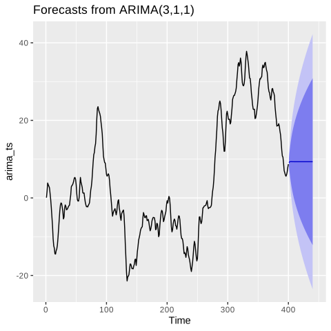
Figure 7.20: forecast of the ARIMA model in R

The central forecast continues the last movement of the series, and the confidence band widens as the horizon increases. This widening is the direct consequence of the unit root: since the shocks never fade, the uncertainty accumulates instead of stabilizing.

In Python:

if 'arima_py' not in globals():
  arima_py = r.arima_ts

arima_fit_py = ARIMA(arima_py, order=(1, 1, 1)).fit()
fc = arima_fit_py.get_forecast(steps=40)
mean_fc = fc.predicted_mean
ci = fc.conf_int()

plt.figure(figsize=(6, 3))

#> <Figure size 600x300 with 0 Axes>

plt.plot(range(len(arima_py)), arima_py, color="black", linewidth=0.8, label="observed")

#> [<matplotlib.lines.Line2D object at 0x0000020E9CF02FC0>]

idx = range(len(arima_py), len(arima_py) + 40)
plt.plot(idx, mean_fc, color="blue", label="forecast")

#> [<matplotlib.lines.Line2D object at 0x0000020E9CE45F10>]

plt.fill_between(idx, ci[:, 0], ci[:, 1], color="blue", alpha=0.2)

#> <matplotlib.collections.PolyCollection object at 0x0000020E9CCE3170>

plt.legend()

#> <matplotlib.legend.Legend object at 0x0000020E9CBDB680>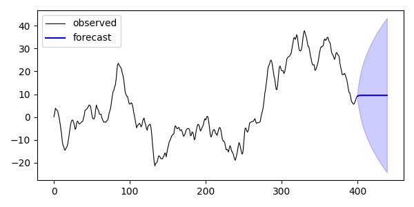

plt.tight_layout()
plt.savefig("arima_fc_py.png")
plt.clf()
plt.close()

Figure 7.21: forecast of the ARIMA model in python

The two forecasts, and the two confidence bands, have the same shape.

7.3.6 ARIMAX model

Everything we have done so far uses only the past of the series to explain its present. In economics we often have an additional variable that we believe to influence the one we study: the temperature for the consumption of electricity, the price for a quantity demanded, a dummy variable for a change of regulation. The \(ARIMAX\) model adds these exogenous regressors to the equation:

\[\begin{equation} \Phi(D)(1-D)^dy_t=\beta^tx_t+\Theta(D)\varepsilon_t \tag{7.37} \end{equation}\]

The coefficient \(\beta\) is read as in a classical regression, and the \(ARIMA\) part now describes what remains once the effect of \(x_t\) has been removed. This is in fact the more honest way of running a regression on time series data: the dynamic structure is modelled explicitly instead of being left in the errors, where it would invalidate the standard errors as we saw in the chapter on the assumptions on the disturbances.

In R:

set.seed(123)
n <- 300

# an exogenous variable and a series that depends on it
x_exo <- rnorm(n, mean = 10, sd = 2)
y_exo <- 5 + 1.5 * x_exo + as.numeric(arima.sim(model = list(ar = 0.7), n = n))

# the exogenous variable is passed through the argument xreg
arimax_fit <- Arima(y_exo, order = c(1, 0, 0), xreg = x_exo)

arimax_out <- data.frame(
  coefficient = names(arimax_fit$coef),
  estimate    = as.numeric(arimax_fit$coef),
  std_error   = sqrt(diag(arimax_fit$var.coef))
)

Table 7.14: estimation of an ARIMAX in R
	coefficient	estimate	std_error
ar1	ar1	0.6217	0.0454
intercept	intercept	4.8681	0.2934
xreg	xreg	1.5134	0.0251

The coefficient attached to the exogenous variable is close to the \(1.5\) used in the simulation, and the auto-regressive coefficient recovers the \(0.7\) of the errors.

In Python:

The same model is obtained by giving the exogenous variable to the argument exog.

if 'x_exo_py' not in globals():
  x_exo_py = r.x_exo
if 'y_exo_py' not in globals():
  y_exo_py = r.y_exo


arimax_fit_py = ARIMA(y_exo_py, exog=np.asarray(x_exo_py), order=(1, 0, 0)).fit()

arimax_out_py = pd.DataFrame({
    "coefficient": ["const", "x_exo", "ar.L1", "sigma2"],
    "estimate": [round(v, 4) for v in arimax_fit_py.params],
    "std_error": [round(v, 4) for v in arimax_fit_py.bse]
})

Table 7.15: estimation of an ARIMAX in python
coefficient	estimate	std_error
const	4.8682	0.2903
x_exo	1.5134	0.0237
ar.L1	0.6217	0.0467
sigma2	0.9543	0.0780

7.3.7 SARIMA model

Many economic series repeat themselves every year, every quarter or every week. Differencing once removes the trend but leaves this repetition untouched, and the correlogram of the differenced series still shows large spikes at the seasonal lags. The \(SARIMA\) model handles them with a second set of orders that work on the seasonal lag \(m\) instead of the lag one:

\[\begin{equation} \Phi(D)\Phi_s(D^m)(1-D)^d(1-D^m)^Dy_t=\Theta(D)\Theta_s(D^m)\varepsilon_t \tag{7.38} \end{equation}\]

It is usually written \(ARIMA(p,d,q)(P,D,Q)_m\), where the capital letters are the seasonal counterparts of the small ones, and \(m\) is the number of periods in a cycle: \(12\) for monthly data, \(4\) for quarterly data. The term \((1-D^m)\) is the seasonal difference, which subtracts from each observation the one of the same period of the previous cycle.

To illustrate it we use the data set AirPassengers, available in R, which gives the monthly number of passengers of an airline between 1949 and 1960. It is the classical example of a series that has at the same time a trend and a seasonality whose amplitude grows with the level, which is why we work on its logarithm.

In R:

data(AirPassengers)
lap <- log(AirPassengers)

par(mfrow = c(1, 2))
plot(AirPassengers, main = "AirPassengers", ylab = "")
plot(lap, main = "log(AirPassengers)", ylab = "")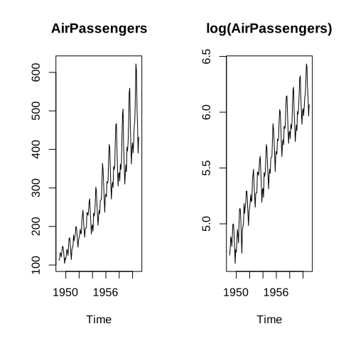

Figure 7.22: the AirPassengers series and its logarithm

par(mfrow = c(1, 1))

The logarithm stabilizes the amplitude of the seasonal oscillations, which is exactly the condition needed for an additive model.

# one ordinary difference and one seasonal difference
Acf(diff(diff(lap), lag = 12), main = "ACF of the twice differenced series")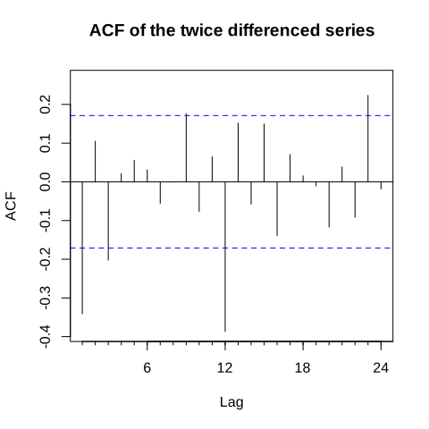

Figure 7.23: correlogram after a seasonal difference

sarima_fit <- auto.arima(lap, seasonal = TRUE, stepwise = FALSE, approximation = FALSE)
sarima_fit

#> Series: lap 
#> ARIMA(0,1,1)(0,1,1)[12] 
#> 
#> Coefficients:
#>           ma1     sma1
#>       -0.4018  -0.5569
#> s.e.   0.0896   0.0731
#> 
#> sigma^2 = 0.001371:  log likelihood = 244.7
#> AIC=-483.4   AICc=-483.21   BIC=-474.77

The selected model is the famous airline model, \(ARIMA(0,1,1)(0,1,1)_{12}\), which Box and Jenkins obtained on this very series.

autoplot(forecast(sarima_fit, h = 36))

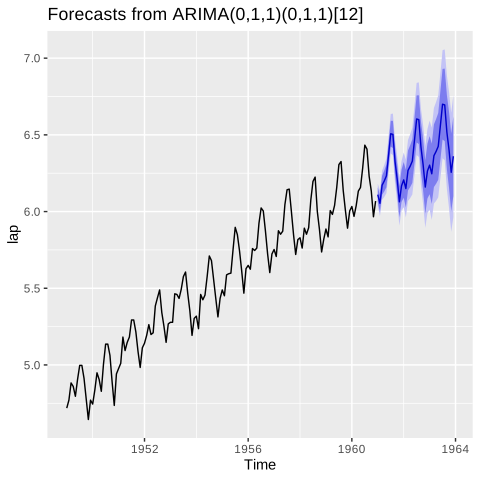
Figure 7.24: forecast of the SARIMA model in R

Contrary to the forecast of the previous section, the seasonal pattern is reproduced in the future, and the confidence band grows much more slowly because a large part of the variability is explained by the season.

In Python:

The class SARIMAX accepts the seasonal orders through the argument seasonal_order, given as \((P,D,Q,m)\).

if 'lap_py' not in globals():
  lap_py = r.lap

from statsmodels.tsa.statespace.sarimax import SARIMAX

sarima_py = SARIMAX(np.asarray(lap_py), order=(0, 1, 1),
                    seasonal_order=(0, 1, 1, 12)).fit(disp=False)

fc_s = sarima_py.get_forecast(steps=36)
ci_s = fc_s.conf_int()

plt.figure(figsize=(6, 3))

#> <Figure size 600x300 with 0 Axes>

plt.plot(range(len(lap_py)), lap_py, color="black", linewidth=0.8, label="observed")

#> [<matplotlib.lines.Line2D object at 0x0000020E9CD25220>]

idx = range(len(lap_py), len(lap_py) + 36)
plt.plot(idx, fc_s.predicted_mean, color="blue", label="forecast")

#> [<matplotlib.lines.Line2D object at 0x0000020E9CED9D90>]

plt.fill_between(idx, ci_s[:, 0], ci_s[:, 1], color="blue", alpha=0.2)

#> <matplotlib.collections.PolyCollection object at 0x0000020E9CCBF230>

plt.legend()

#> <matplotlib.legend.Legend object at 0x0000020E9CE8E8A0>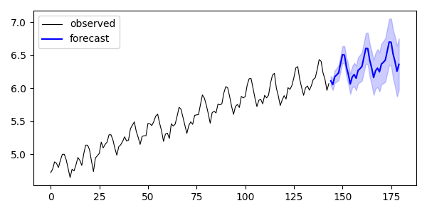

plt.tight_layout()
plt.savefig("sarima_fc_py.png")
plt.clf()
plt.close()

Figure 7.25: forecast of the SARIMA model in python


sarima_out_py = pd.DataFrame({
    "coefficient": ["ma.L1", "ma.S.L12", "sigma2"],
    "estimate": [round(v, 4) for v in sarima_py.params],
    "std_error": [round(v, 4) for v in sarima_py.bse]
})

Table 7.16: estimation of the airline model in python
coefficient	estimate	std_error
ma.L1	-0.4021	0.0730
ma.S.L12	-0.5568	0.0963
sigma2	0.0013	0.0001

The two coefficients are very close to those returned by auto.arima, and the two forecasts are indistinguishable.