7.7 Multivariate time series
Everything we have done until now had one variable on the left hand side and, at best, a few exogenous regressors on the right hand side. This asymmetry requires us to decide in advance which variable explains which, and that decision comes from outside the data. Sims objected in 1980 that this choice is often arbitrary, that the large simultaneous equation models of the time rested on restrictions that nobody really believed, and he proposed to abandon the distinction between endogenous and exogenous variables altogether.
The vector autoregression that he introduced treats all the variables symmetrically: each of them is explained by its own past and by the past of all the others. Nothing is imposed beforehand except the number of lags, and the data are left to say what depends on what.
7.7.1 VAR models
Let \(y_t\) be a vector of \(g\) variables observed at the same dates. The \(VAR(p)\) writes:
\[\begin{equation} y_t=c+A_1y_{t-1}+A_2y_{t-2}+...+A_py_{t-p}+u_t \tag{7.49} \end{equation}\]
where each \(A_i\) is a square matrix of dimension \(g\) and \(u_t\) is a vector of errors with variance matrix \(\Sigma\). For two variables and one lag the system is simply:
\[\begin{align} y_{1t}&=c_1+a_{11}y_{1,t-1}+a_{12}y_{2,t-1}+u_{1t} \\ y_{2t}&=c_2+a_{21}y_{1,t-1}+a_{22}y_{2,t-1}+u_{2t} \end{align}\]
Two remarks follow immediately from this writing. First, every equation contains exactly the same regressors, so the generalized least squares bring nothing and the system can be estimated equation by equation by ordinary least squares, which stays consistent and efficient. Second, the number of coefficients grows very fast: a model with \(g\) variables and \(p\) lags contains \(g(gp+1)\) coefficients, that is \(84\) for six variables and two lags. This is the main practical limit of the approach, and the reason why the lag order must be chosen with care, using the information criteria as we did for the univariate models.
The stationarity condition generalizes the one of the \(AR(p)\): the process is stationary if all the eigenvalues of the companion matrix have a modulus smaller than one, or equivalently if the roots of \(\det(I-A_1D-...-A_pD^p)=0\) lie outside the unit circle.
Let us simulate a stationary bivariate system and estimate it.
In R:
set.seed(123)
n <- 500

# the true coefficient matrix
A <- matrix(c(0.5, 0.2,
              0.1, 0.6), nrow = 2, byrow = TRUE)

Y <- matrix(0, nrow = n, ncol = 2)
for (t in 2:n) {
  Y[t, ] <- A %*% Y[t - 1, ] + rnorm(2, sd = 1)
}
colnames(Y) <- c("y1", "y2")
var_data <- ts(Y[-(1:50), ])   # we drop the first observations

plot(var_data, main = "the two simulated series")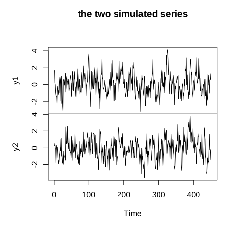
Figure 7.31: a simulated bivariate VAR(1)
The package vars selects the number of lags with four criteria at once and estimates the system.
suppressPackageStartupMessages(library(vars))

# selection of the number of lags
lag_sel <- VARselect(var_data, lag.max = 8, type = "const")
sel_out <- data.frame(criterion = names(lag_sel$selection),
lags = as.integer(lag_sel$selection))| criterion | lags |
|---|---|
| AIC(n) | 1 |
| HQ(n) | 1 |
| SC(n) | 1 |
| FPE(n) | 1 |
The criteria agree on one lag, which is the order we simulated.
var_fit <- VAR(var_data, p = 1, type = "const")

var_coef <- rbind(
  data.frame(equation = "y1", coefficient = rownames(coef(var_fit)$y1),
             estimate = coef(var_fit)$y1[, 1]),
  data.frame(equation = "y2", coefficient = rownames(coef(var_fit)$y2),
             estimate = coef(var_fit)$y2[, 1])
)| equation | coefficient | estimate |
|---|---|---|
| y1 | y1.l1 | 0.5264 |
| y1 | y2.l1 | 0.2210 |
| y1 | const | 0.0748 |
| y2 | y1.l1 | 0.0541 |
| y2 | y2.l1 | 0.5529 |
| y2 | const | -0.0580 |
The estimated coefficients reproduce the matrix \(A\) used in the simulation, with one reservation: the smallest of them, the effect of \(y_1\) on \(y_2\), is recovered with much less precision than the others, and we will see the consequence of it in a moment.
Since the individual coefficients of a \(VAR\) are hard to interpret, three tools are used to read the system.
The first one is the Granger causality. We say that \(y_2\) causes \(y_1\) in the sense of Granger if the past of \(y_2\) helps to predict \(y_1\) once the past of \(y_1\) is already taken into account. This is a statement about predictability, not about causality in the ordinary meaning of the word, and the vocabulary has caused a great deal of confusion.
g1 <- causality(var_fit, cause = "y2")$Granger
g2 <- causality(var_fit, cause = "y1")$Granger

granger_out <- data.frame(
  hypothesis = c("y2 does not cause y1", "y1 does not cause y2"),
  statistic  = c(g1$statistic, g2$statistic),
  p_value    = c(g1$p.value, g2$p.value)
)| hypothesis | statistic | p_value |
|---|---|---|
| y2 does not cause y1 | 32.0359 | 0.0000 |
| y1 does not cause y2 | 1.9377 | 0.1643 |
The first hypothesis is clearly rejected: the past of \(y_2\) does help to predict \(y_1\). The second one, on the contrary, is not rejected at the usual levels, although we did put a coefficient \(a_{21}=0.1\) in the simulation. The effect exists, but it is small relative to the variance of the shocks and the sample is not long enough to separate it from zero. This is worth remembering before concluding from a non rejection that there is no relation: the test tells us what the data can detect, not what the world contains. Here the causality in the sense of Granger is therefore found in one direction only.
The second tool is the impulse response function, generalized to the multivariate case, which traces the reaction of every variable to a shock on any of them. The third is the variance decomposition, which gives the share of the forecast error variance of each variable attributable to each shock.
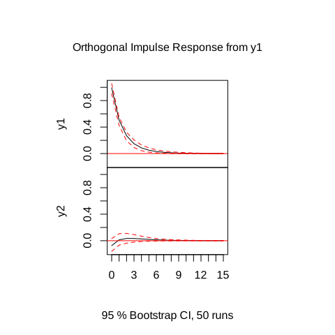
Figure 7.32: impulse responses of the VAR in R
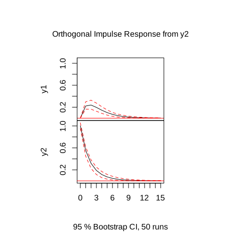
Figure 7.33: impulse responses of the VAR in R
| horizon | y1 | y2 |
|---|---|---|
| 1 | 1.0000 | 0.0000 |
| 2 | 0.9618 | 0.0382 |
| 3 | 0.9249 | 0.0751 |
| 4 | 0.9019 | 0.0981 |
| 5 | 0.8898 | 0.1102 |
| 6 | 0.8839 | 0.1161 |
At the first horizon the whole forecast error of \(y_1\) comes from its own shock, and the contribution of the shock on \(y_2\) grows with the horizon, which is the way the transmission between the two variables shows itself.
In Python:
The statsmodels package provides the same model through the class VAR.
from statsmodels.tsa.api import VAR

var_arr = np.asarray(var_py, dtype=float)
var_fit_py = VAR(var_arr).fit(maxlags=1, ic=None, trend="c")

var_out_py = pd.DataFrame(np.round(var_fit_py.params, 4),
                          columns=["y1", "y2"])
var_out_py.insert(0, "coefficient", ["const", "L1.y1", "L1.y2"])| coefficient | y1 | y2 |
|---|---|---|
| const | 0.0748 | -0.0580 |
| L1.y1 | 0.5264 | 0.0541 |
| L1.y2 | 0.2210 | 0.5529 |
The coefficients are the same as those obtained in R, read column by column.
7.7.1.1 Reduced form
The model of equation (7.49) is the reduced form of the system. Its defining feature is that it contains no contemporaneous variable on the right hand side: \(y_{1t}\) is explained by \(y_{1,t-1}\) and \(y_{2,t-1}\), never by \(y_{2t}\). This is what makes the estimation so simple, since each equation satisfies the conditions of the ordinary least squares.
The price of this simplicity appears in the errors. The vector \(u_t\) has in general a variance matrix \(\Sigma\) that is not diagonal, which means that the two errors move together within the same period. Economically this is not surprising: if the two variables react simultaneously to a common event, the part of that event which is not explained by the past ends up in both errors at once.
#>        y1     y2
#> y1  1.000 -0.074
#> y2 -0.074  1.000
The consequence is important for the interpretation. We cannot speak of “a shock on \(y_1\) alone”, because a movement of \(u_{1t}\) is on average accompanied by a movement of \(u_{2t}\). The errors of the reduced form are statistical residuals, not economic shocks, and the impulse responses computed directly on them would mix several causes. To recover interpretable shocks we need the structural form.
7.7.1.2 Structural form
The structural form writes the system with its contemporaneous relations explicit:
\[\begin{equation} B_0y_t=c+B_1y_{t-1}+...+B_py_{t-p}+\varepsilon_t \tag{7.50} \end{equation}\]
where the matrix \(B_0\) carries the instantaneous effects of the variables on each other, and where the structural shocks \(\varepsilon_t\) are, by construction, mutually uncorrelated: each of them has its own economic meaning, a demand shock, a monetary shock, and so on. Multiplying by \(B_0^{-1}\) gives back the reduced form, with:
\[\begin{equation} u_t=B_0^{-1}\varepsilon_t \quad \text{and} \quad \Sigma=B_0^{-1}\Omega (B_0^{-1})^t \tag{7.51} \end{equation}\]
Here lies the identification problem. The estimation gives us \(\Sigma\), which is symmetric and therefore contains \(\frac{g(g+1)}{2}\) distinct numbers, while \(B_0\) and the variances of the structural shocks together contain \(g^2\) unknowns. There are more unknowns than equations, and we must impose \(\frac{g(g-1)}{2}\) restrictions from outside the data.
The most common choice is the Cholesky decomposition, which imposes that \(B_0^{-1}\) is lower triangular. This amounts to ordering the variables and assuming that the first one is not affected within the period by the shocks on the following ones, while it may affect them immediately. The ordering is therefore an economic assumption, and not a technical detail: reversing it changes the responses, and any serious work reports the sensitivity of the conclusions to that choice.
In R:
# ortho = TRUE applies the Cholesky decomposition with the current ordering
irf_ortho <- irf(var_fit, impulse = "y1", response = c("y1", "y2"),
                 n.ahead = 15, ortho = TRUE, boot = TRUE, runs = 50)
plot(irf_ortho)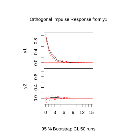
Figure 7.34: orthogonalized impulse responses in R
The response of \(y_2\) to a structural shock on \(y_1\) is now interpretable, because the shock has been purged of its contemporaneous correlation with the other error.
The Cholesky ordering is not the only possible identification. The literature also uses long run restrictions, which impose that certain shocks have no permanent effect, and sign restrictions, which only require the responses to have an expected sign during a few periods. All of them share the same logic: the data alone cannot separate the structural shocks, and the separation must come from the theory.
In Python:
irf_py = var_fit_py.irf(15)

fig = irf_py.plot(orth=True, impulse=0)
fig.set_size_inches(7, 4)
plt.tight_layout()
plt.savefig("var_irf_py.png")
plt.clf()
plt.close()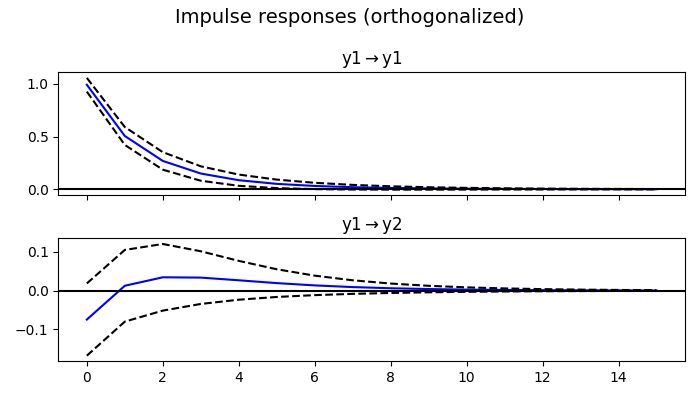
Figure 7.35: orthogonalized impulse responses in python
7.7.2 VECM models
The \(VAR\) of the previous sections requires stationary variables. When the series are \(I(1)\) we are back to the dilemma of the cointegration section, but this time for a whole system: estimating the \(VAR\) on the levels gives inconsistent inference, and estimating it on the differences throws away the long run relations.
The vector error correction model is the multivariate answer, and it is exactly the generalization of the error correction model to \(g\) variables. Starting from a \(VAR(p)\) on \(I(1)\) variables and rearranging the terms, we obtain:
\[\begin{equation} \vartriangle y_t=\Pi y_{t-1}+\sum_{i=1}^{p-1}\Gamma_i \vartriangle y_{t-i}+u_t \tag{7.52} \end{equation}\]
Everything in this equation is stationary except possibly the term \(\Pi y_{t-1}\), and the whole content of the analysis is in the rank of the matrix \(\Pi\):
if \(rank(\Pi)=0\), the matrix is null, there is no cointegrating relation and the correct model is a \(VAR\) on the differences;
if \(rank(\Pi)=g\), the matrix has full rank and the variables were in fact stationary in level, so a \(VAR\) on the levels was appropriate from the start;
if \(0<rank(\Pi)=r<g\), there are exactly \(r\) cointegrating relations, and the matrix factorizes as \(\Pi=\alpha\beta^t\) where \(\beta\) contains the \(r\) long run relations and \(\alpha\) the speeds of adjustment.
The columns of \(\beta\) play the role of the vector \((1,-\beta)\) of the bivariate case, and the coefficients of \(\alpha\) are the multivariate counterparts of the \(\lambda\) of the error correction model: they say how each variable reacts to each disequilibrium.
7.7.2.1 Johansen Methodology
Determining the rank \(r\) is therefore the central question, and it is what the Johansen procedure does. The method estimates the system by maximum likelihood and computes the \(g\) eigenvalues \(\lambda_1>\lambda_2>...>\lambda_g\) associated with the matrix \(\Pi\). The rank is the number of eigenvalues that are significantly different from zero, and two statistics are used to count them. Both are applied in sequence, starting from \(r=0\) and stopping at the first hypothesis that is not rejected.
Johansen’s trace statistic:
This statistic tests the null hypothesis that there are at most \(r\) cointegrating relations against the alternative that there are more. It gathers all the eigenvalues beyond the rank \(r\):
\[\begin{equation} \lambda_{trace}(r)=-T\sum_{i=r+1}^{g}\ln(1-\hat\lambda_i) \tag{7.53} \end{equation}\]
If the remaining eigenvalues are all close to zero, the logarithms are close to zero as well and the statistic is small, which leads to accepting the rank \(r\).
Maximum eigenvalue statistic:
This one tests the null hypothesis of exactly \(r\) relations against the precise alternative of \(r+1\), and uses only the next eigenvalue:
\[\begin{equation} \lambda_{max}(r,r+1)=-T\ln(1-\hat\lambda_{r+1}) \tag{7.54} \end{equation}\]
Being more specific in its alternative, it is often more powerful, but the two statistics may disagree, in which case the trace is usually preferred because its sequence of tests is coherent.
Let us apply the procedure to the two cointegrated series built in the cointegration section, for which we know that there is exactly one long run relation.
In R:
The function ca.jo of the package urca performs both tests.
coint_data <- cbind(y = as.numeric(y_co), x = as.numeric(x_co))

jo_trace <- ca.jo(coint_data, type = "trace", ecdet = "const", K = 2)
summary(jo_trace)
#>
#> ######################
#> # Johansen-Procedure #
#> ######################
#>
#> Test type: trace statistic , without linear trend and constant in cointegration
#>
#> Eigenvalues (lambda):
#> [1] 3.599759e-01 1.178933e-02 -1.003200e-17
#>
#> Values of teststatistic and critical values of test:
#>
#> test 10pct 5pct 1pct
#> r <= 1 | 4.72 7.52 9.24 12.97
#> r = 0 | 182.33 17.85 19.96 24.60
#>
#> Eigenvectors, normalised to first column:
#> (These are the cointegration relations)
#>
#> y.l2 x.l2 constant
#> y.l2 1.000000 1.0000000 1.0000000
#> x.l2 -1.493204 0.4150832 0.9041317
#> constant -2.042228 -10.7034054 42.0953630
#>
#> Weights W:
#> (This is the loading matrix)
#>
#> y.l2 x.l2 constant
#> y.d -0.2851520 -0.01890255 -1.244654e-17
#> x.d 0.5178345 -0.01287282 2.515204e-17The reading follows the sequence. The first line, \(r=0\), has a statistic far above its critical value, so the absence of cointegration is rejected. The second line, \(r\leqslant 1\), has a statistic below its critical value, so we stop there and conclude that the rank is one: there is exactly one cointegrating relation, which is what we built.
jo_max <- ca.jo(coint_data, type = "eigen", ecdet = "const", K = 2)

# urca returns the hypotheses from the largest rank to the smallest, so we
# reverse them to read the sequence in the natural order, starting at r = 0.
ord <- rev(seq_along(jo_trace@teststat))

jo_out <- data.frame(
  hypothesis = rownames(jo_max@cval)[ord],
  trace_stat = as.numeric(jo_trace@teststat)[ord],
  eigen_stat = as.numeric(jo_max@teststat)[ord],
  crit_5pct  = as.numeric(jo_max@cval[, "5pct"])[ord]
)| hypothesis | trace_stat | eigen_stat | crit_5pct |
|---|---|---|---|
| r = 0 | | 182.327 | 177.607 | 15.67 |
| r <= 1 | | 4.720 | 4.720 | 9.24 |
The two statistics give the same answer here.
Once the rank is known, the system can be estimated and converted into a \(VAR\) representation for forecasting.
# the cointegrating vector, normalized on the first variable
beta_hat <- jo_trace@V[, 1] / jo_trace@V[1, 1]
round(beta_hat, 4)
#> y.l2 x.l2 constant
#> 1.0000 -1.4932 -2.0422The coefficient attached to \(x\) is again close to the value used in the simulation, up to the sign convention: the relation is written \(y-1.5x\approx const\), so the coefficient appears with a negative sign in the normalized vector.
In Python:
The module statsmodels.tsa.vector_ar.vecm provides the function coint_johansen for the rank tests and the class VECM for the estimation.
from statsmodels.tsa.vector_ar.vecm import coint_johansen, VECM

coint_arr = np.column_stack([np.asarray(y_co_py, dtype=float),
                             np.asarray(x_co_py, dtype=float)])

jo = coint_johansen(coint_arr, det_order=0, k_ar_diff=1)

jo_py = pd.DataFrame({
    "hypothesis": ["r = 0", "r <= 1"],
    "trace_stat": np.round(jo.lr1, 3),
    "trace_crit_5pct": np.round(jo.cvt[:, 1], 3),
    "eigen_stat": np.round(jo.lr2, 3),
    "eigen_crit_5pct": np.round(jo.cvm[:, 1], 3)
})| hypothesis | trace_stat | trace_crit_5pct | eigen_stat | eigen_crit_5pct |
|---|---|---|---|---|
| r = 0 | 182.139 | 15.494 | 177.606 | 14.264 |
| r <= 1 | 4.533 | 3.842 | 4.533 | 3.842 |
vecm_py = VECM(coint_arr, k_ar_diff=1, coint_rank=1, deterministic="ci").fit()

vecm_out_py = pd.DataFrame({
    "quantity": ["beta (normalized on y)", "beta (x)",
                 "alpha (adjustment of y)", "alpha (adjustment of x)"],
    "value": [round(float(vecm_py.beta[0, 0]), 4),
              round(float(vecm_py.beta[1, 0]), 4),
              round(float(vecm_py.alpha[0, 0]), 4),
              round(float(vecm_py.alpha[1, 0]), 4)]
})| quantity | value |
|---|---|
| beta (normalized on y) | 1.0000 |
| beta (x) | -1.4932 |
| alpha (adjustment of y) | -0.2852 |
| alpha (adjustment of x) | 0.5178 |
The cointegrating vector is normalized on the first variable, and the adjustment coefficient of \(y\) is negative, which means that when \(y\) is above its long run relation with \(x\) it is pushed back downwards, exactly as in the bivariate error correction model of the previous section.
With this last model we have covered the whole path of the chapter. We started from a single series and its components, we learned to recognize whether it is stationary and to make it so, we modelled its mean with the \(ARIMA\) family and its variance with the \(GARCH\) family, and we finally moved to several series at once, first without long run relation with the \(VAR\), then with one through the \(VECM\). The next chapter leaves this framework and asks what machine learning algorithms can add when the relations between the variables are too complex to be written as a linear system.