9.6 Recurrent neural networks
We now change the structure being exploited: no longer space, but time. The models of this section read a sequence element by element while carrying a memory of what came before, which connects them directly to the time series of chapter seven. We end by putting the two approaches side by side on the same series.
9.6.1 Sequential data
The convolutional network exploited a structure in space. A recurrent network exploits a structure in time: the observations arrive in an order, that order carries meaning, and the sequences do not all have the same length.
The networks seen so far cannot handle this. A dense layer requires a fixed number of inputs, so a sentence of ten words and one of forty cannot be fed to the same model without padding or truncating. And it treats the positions as independent coordinates, so nothing tells it that position \(t\) comes just after position \(t-1\).
One could of course build a window of fixed size and feed the last \(k\) values, which is exactly what the autoregressive models of chapter seven do. The limitation is the same as theirs: the memory stops at \(k\), and enlarging \(k\) enlarges the model. A recurrent network keeps instead a state that it carries from one step to the next, and whose size does not depend on the length of the sequence.
9.6.2 The recurrent cell
The cell reads the sequence one element at a time. At each step it combines the current input with the state inherited from the previous step, and produces a new state:
\[\begin{align} h_t&=g\big(W_{h}h_{t-1}+W_{x}x_t+b\big) \\ \hat y_t&=W_{y}h_t+b_y \tag{9.21} \end{align}\]
Everything of importance is in the first line. The state \(h_t\) is a summary of everything read so far, and the matrices \(W_h\), \(W_x\), \(b\) are the same at every step: this is weight sharing again, in time rather than in space, and it is what allows a single model to process sequences of any length.
The usual way of drawing this is to unroll the cell over the length of the sequence, which turns the loop into a deep network whose layers all share their weights.
In R:
steps_n <- 5
cells <- data.frame(t = 1:steps_n, x = 1:steps_n, y = 1)

ggplot() +
  geom_segment(data = data.frame(x = 1:(steps_n - 1)),
               aes(x = x + .22, xend = x + .78, y = 1, yend = 1),
               arrow = arrow(length = unit(.18, "cm")), colour = "grey45") +
  geom_segment(data = cells, aes(x = x, xend = x, y = .55, yend = .82),
               arrow = arrow(length = unit(.15, "cm")), colour = "grey45") +
  geom_segment(data = cells, aes(x = x, xend = x, y = 1.18, yend = 1.45),
               arrow = arrow(length = unit(.15, "cm")), colour = "grey45") +
  geom_point(data = cells, aes(x, y), shape = 21, size = 20,
             fill = "steelblue", alpha = .25, colour = "steelblue") +
  geom_text(data = cells, aes(x, y, label = paste0("h", t)), size = 3.2) +
  geom_text(data = cells, aes(x, .45, label = paste0("x", t)), size = 3.2) +
  geom_text(data = cells, aes(x, 1.55, label = paste0("y", t)), size = 3.2) +
  xlim(.4, steps_n + .6) + ylim(.3, 1.7) +
  labs(title = "an unrolled recurrent cell",
       subtitle = "the same weights are used at every step") +
  theme_void() + theme(plot.subtitle = element_text(size = 9))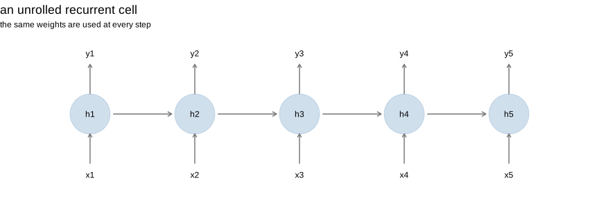
Figure 9.25: the same cell, drawn as a loop and unrolled in time
9.6.3 Backpropagation through time
Training uses the same backpropagation as before, applied to the unrolled network, which is called backpropagation through time. The gradient of the loss at step \(t\) travels back through every earlier step, and at each of them it is multiplied by the same matrix \(W_h\) and by the derivative of the activation.
That repetition is the whole difficulty. Going back \(k\) steps multiplies the gradient by roughly \(W_h^k\), so the behaviour is governed by the largest eigenvalue of \(W_h\): below one the gradient vanishes exponentially, above one it explodes. This is the vanishing gradient of the earlier section, in a particularly severe form, because the same matrix is repeated rather than a sequence of different ones.
The practical consequence is that a simple recurrent cell cannot learn long dependencies. It handles ten steps, struggles at fifty, and is hopeless at five hundred.
In R:
set.seed(1)
horizon <- 60

decay <- function(lambda, label) {
  W <- diag(lambda, 12)                       # a state matrix with a known scale
  d <- matrix(rnorm(12), 1, 12)
  nr <- numeric(horizon)
  for (k in 1:horizon) {
    d <- d %*% W * 0.9                        # 0.9 stands for the activation derivative
    nr[k] <- sqrt(sum(d^2))
  }
  data.frame(step_back = 1:horizon, norm = nr, regime = label)
}

grad_time <- rbind(decay(0.8, "largest eigenvalue < 1 (vanishing)"),
                   decay(1.0, "largest eigenvalue = 1"),
                   decay(1.2, "largest eigenvalue > 1 (exploding)"))

ggplot(grad_time, aes(step_back, norm, colour = regime)) +
  geom_line(linewidth = .9) + scale_y_log10() +
  labs(title = "norm of the gradient as it travels back in time",
       x = "number of steps back", y = "norm (log scale)") +
  theme_minimal() + theme(legend.position = "bottom")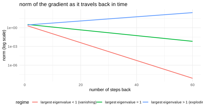
Figure 9.26: how far back the gradient survives
The vertical scale is logarithmic, so the straight lines are exponentials. In the first regime the gradient has lost twenty orders of magnitude after sixty steps, meaning the network cannot possibly connect an event to a consequence sixty steps later. In the third it has gained as many, which in practice returns NaN within a few updates.
9.6.4 LSTM and GRU
The long short-term memory cell was designed to break that exponential. Its key idea is to add a cell state \(C_t\) that is modified by additions rather than by repeated matrix multiplications, so that information can travel along it almost unchanged. Three gates, each a small sigmoid layer producing values between zero and one, decide what happens:
\[\begin{align} f_t&=\sigma\big(W_f[h_{t-1},x_t]+b_f\big) &&\text{forget: what to erase from } C_{t-1} \\ i_t&=\sigma\big(W_i[h_{t-1},x_t]+b_i\big) &&\text{input: what to write} \\ \tilde C_t&=\tanh\big(W_C[h_{t-1},x_t]+b_C\big) &&\text{the candidate content} \\ C_t&=f_t\odot C_{t-1}+i_t\odot\tilde C_t &&\text{the update, additive} \\ o_t&=\sigma\big(W_o[h_{t-1},x_t]+b_o\big) &&\text{output: what to expose} \\ h_t&=o_t\odot\tanh(C_t) \tag{9.22} \end{align}\]
The line that matters is the fourth. When the forget gate is close to one and the input gate close to zero, \(C_t\approx C_{t-1}\): the state passes through untouched, and so does the gradient. The network can therefore learn to keep a piece of information for hundreds of steps, and equally learn to drop it when the forget gate closes.
The GRU is a simplification with two gates instead of three and no separate cell state. It has fewer parameters, trains a little faster, and performs comparably in most applications; the choice between the two is usually made empirically.
In R:
set.seed(3)
Tn <- 40
gates <- data.frame(
  t = rep(1:Tn, 3),
  value = c(c(rep(.95, 15), rep(.1, 5), rep(.95, 20)),      # forget
            c(rep(.1, 12), rep(.9, 6), rep(.15, 22)),        # input
            c(rep(.5, 8), rep(.9, 24), rep(.3, 8))),         # output
  gate = rep(c("forget", "input", "output"), each = Tn))

ggplot(gates, aes(t, value, colour = gate)) +
  geom_line(linewidth = .9) + ylim(0, 1) +
  labs(title = "an illustration of the three gates over a sequence",
       subtitle = "forget near 1 keeps the memory; input near 1 writes into it",
       x = "time step", y = "gate value") +
  theme_minimal()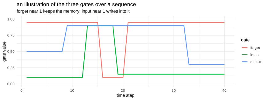
Figure 9.27: the gates of an LSTM control what is kept
This figure is an illustration rather than a measurement, but it shows the logic. While the forget gate stays near one and the input gate near zero, the cell preserves what it holds. Around the twelfth step the input gate opens and new information is written. Later the forget gate drops briefly, which erases the memory and starts afresh.
9.6.5 Application to a time series
We return to the series of airline passengers used in the time series chapter, and we ask a recurrent network to forecast it. This allows a direct comparison with the \(SARIMA\) model obtained there.
The preparation is specific to this kind of model and deserves attention. The series is cut into overlapping windows: the input is a block of twelve consecutive months, the target is the following month. The data must also be scaled, because a recurrent network handles values near zero much better, and the split between training and test must respect the chronological order, since shuffling would let the model learn from the future.
In Python:
The series is reloaded here so that this chapter does not depend on the state left by the previous one.
#> <torch._C.Generator object at 0x0000020E2AABD510>series = np.asarray(lap_dl_py, dtype="float32")
# scaling is fitted on the training part only
n_test = 24
train_raw = series[:-n_test]
mu, sd = train_raw.mean(), train_raw.std()
scaled = (series - mu) / sd
L = 12
def windows(x, L):
X = np.stack([x[i:i+L] for i in range(len(x) - L)])
y = x[L:]
return X[:, :, None].astype("float32"), y.astype("float32")
Xseq, yseq = windows(scaled, L)
split = len(Xseq) - n_test
Xs_tr = torch.tensor(Xseq[:split]); ys_tr = torch.tensor(yseq[:split]).view(-1, 1)
Xs_te = torch.tensor(Xseq[split:]); ys_te = torch.tensor(yseq[split:]).view(-1, 1)
class Recurrent(nn.Module):
def __init__(self, kind="LSTM", hidden=32):
super().__init__()
cell = {"RNN": nn.RNN, "LSTM": nn.LSTM, "GRU": nn.GRU}[kind]
self.rnn = cell(input_size=1, hidden_size=hidden, batch_first=True)
self.out = nn.Linear(hidden, 1)
def forward(self, x):
o, _ = self.rnn(x)
return self.out(o[:, -1, :]) # only the last state is used
def fit_seq(model, epochs=400, lr=1e-2):
opt = torch.optim.Adam(model.parameters(), lr=lr)
lf = nn.MSELoss()
for _ in range(epochs):
opt.zero_grad()
lf(model(Xs_tr), ys_tr).backward()
opt.step()
return model
results_seq = []
preds = {}
for kind in ["RNN", "LSTM", "GRU"]:
torch.manual_seed(0)
m = fit_seq(Recurrent(kind))
m.eval()
with torch.no_grad():
p = m(Xs_te).numpy().ravel()
preds[kind] = p * sd + mu # back to the original scale
truth = yseq[split:] * sd + mu
rmse = float(np.sqrt(np.mean((preds[kind] - truth) ** 2)))
results_seq.append({"model": kind, "test_RMSE": round(rmse, 4)})#> <torch._C.Generator object at 0x0000020E2AABD510>
#> Recurrent(
#> (rnn): RNN(1, 32, batch_first=True)
#> (out): Linear(in_features=32, out_features=1, bias=True)
#> )
#> <torch._C.Generator object at 0x0000020E2AABD510>
#> Recurrent(
#> (rnn): LSTM(1, 32, batch_first=True)
#> (out): Linear(in_features=32, out_features=1, bias=True)
#> )
#> <torch._C.Generator object at 0x0000020E2AABD510>
#> Recurrent(
#> (rnn): GRU(1, 32, batch_first=True)
#> (out): Linear(in_features=32, out_features=1, bias=True)
#> )| model | test_RMSE |
|---|---|
| RNN | 0.1268 |
| LSTM | 0.1617 |
| GRU | 0.1010 |
#> <Figure size 800x340 with 0 Axes>#> [<matplotlib.lines.Line2D object at 0x0000020F2C98D310>]idx_te = range(L + split, L + split + n_test)
for kind, col in zip(["RNN", "LSTM", "GRU"], ["tab:orange", "tab:blue", "tab:green"]):
plt.plot(idx_te, preds[kind], color=col, linewidth=1.1, label=kind)#> [<matplotlib.lines.Line2D object at 0x0000020F2CA3CB60>]
#> [<matplotlib.lines.Line2D object at 0x0000020F2CA3CD10>]
#> [<matplotlib.lines.Line2D object at 0x0000020F2C9F3DD0>]#> <matplotlib.legend.Legend object at 0x0000020F2C8FECC0>#> Text(0.5, 1.0, 'log of the number of passengers')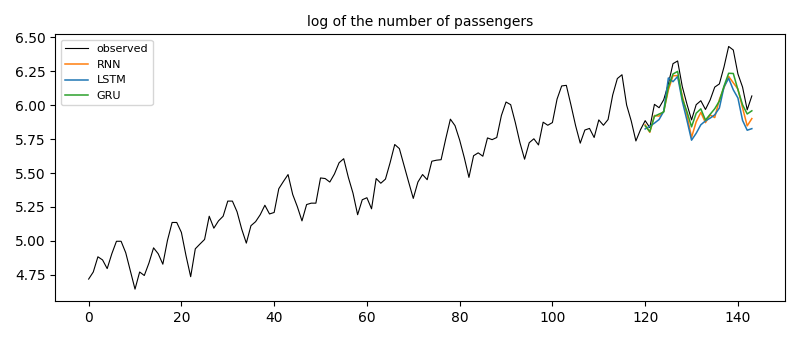
Figure 9.28: recurrent forecasts of the airline series
The three cells follow the seasonal pattern and the trend, which is already a result: nothing in the model was told that the period is twelve, whereas the \(SARIMA\) of chapter seven had to be given that information explicitly through its seasonal orders.
The ranking of the three cells is worth a comment, because it is not the one a reader might expect. The LSTM, the most elaborate of the three, comes last here, and the plain recurrent cell beats it. There is no paradox: the windows are twelve steps long, so there is no long dependency to capture, and the gates that make the LSTM valuable over hundreds of steps are here only additional parameters to estimate on a hundred and twenty observations. A more complex cell helps when the problem needs it, and costs when it does not.
It is worth being clear about what this comparison does and does not show. On a series of a hundred and forty observations, a well specified \(SARIMA\) remains an excellent model, and it has decisive advantages: it is estimated in a fraction of a second, it provides confidence intervals, and its coefficients are interpretable. The recurrent network offers none of these things here. Its advantages appear elsewhere: when the series is long, when several series are modelled together, when exogenous variables of different natures must be mixed, and when the dynamic is too nonlinear to be written as an \(ARIMA\). Choosing a network for a short univariate seasonal series would be a mistake, and it is a common one.