6.3 Non parametric regressions
This method can be a good choice if we have no assumption of the functional form of the model, hence no global parameters to estimate. Therefore, the general model, with one regressor for simplification, should be given by:
\[\begin{equation} y_i=\mathrm g\big(x_i\big)+\varepsilon_i \tag{6.38} \end{equation}\]
As we see this function is free of the parameter \(\beta\).
The basic technique used to estimate the dependent variable with a fixed value \(x^*\) is by taking the average of the neighborhood observations. Determining if an observation \((y_i, x_i)\) is in the neighborhood or not is by checking the difference between those two values \(x_i\) and \(x^*\). If \(|x_i-x^*|\leqslant h\) then this observation will be used in the estimation. The \(h\) is called the bandwidth, and it should be chosen carefully, such that small values lead to smooth curve estimation. However, some practitioners used the common one called Silverman’s rule of thumb:
\[\begin{equation*} h=0.9min\Bigg(\widehat\sigma,\frac{IQR}{1.349}\Bigg)n^{-0.2} \end{equation*}\]
Where \(\widehat\sigma\) is the sample standard deviation and \(IQR\) is the interquartile range.
We can also find the best value for \(h\) using the cross validation technique used widely in machine learning.
Formally, the resulted estimator will be written:
\[\begin{equation} \widehat{\mathrm g}\big(x^*\big)=\frac{\sum\limits_{i=1}^nI_{(|x_i-x^*|\leqslant h)}y_i}{\sum\limits_{i=1}^nI_{(|x_i-x^*|\leqslant h)}} \tag{6.39} \end{equation}\]
Where \(I=1\) if \(|x_i-x^*|\leqslant h\), otherwise \(I=0\).
This basic estimator is called binned mean.
The main shortcomings of this method is that the estimated function is not smooth and behaves like a step function and all the points in the neighborhood are treated equally even when some of which are far from \(x^*\) than others. This give rise to some alternatives that produce a smooth and continuous functions. We will discuss the most used ones.
6.3.1 Local Constant estimator NW
This estimator, also known as Nadarya-Watson estimator (Nadaraya 1964), uses a kernel function to control the smoothness of the estimated function \(\mathrm g\) than The binned estimator, which is a special case of that one.
That estimator is given by:
\[\begin{equation} \widehat{\mathrm g}_{NW}\big(x^*\big)=\frac{\sum\limits_{i=1}^nk\big(x^*|x_i\big)y_i}{\sum\limits_{i=1}^nk\big(x^*|x_i\big)} \tag{6.40} \end{equation}\]
The role of the kernel \(k\) is to give less weight for far points in a declining smoother way. The most used kernels in practice are:
The Gaussian kernel
\[\begin{equation} k\big(x^*|x_i\big)=\frac{1}{h\sqrt{2\pi}}exp\Bigg(-0.5\bigg(\frac{x_i-x^*}{h}\bigg)\Bigg) \tag{6.41} \end{equation}\]
The Logistic kernel:
\[\begin{equation} k\big(x^*|x_i\big)=\Lambda\bigg(\frac{x_i-x^*}{h}\bigg)\bigg[1-\Lambda\bigg(\frac{x_i-x^*}{h}\bigg)\bigg] \tag{6.41} \end{equation}\]
Where \(\Lambda(x)=\frac{exp(x)}{1+exp(x)}\) is the classical logistic function.
The Epanechnikov kernel:
\[\begin{equation} k\big(x^*|x_i\big)=\begin{cases} \frac{0.75\Bigg[1-0.2\bigg(\frac{x_i-x^*}{h}\bigg)^2\Bigg]}{\sqrt 5} \qquad if \qquad \bigg|\frac{x_i-x^*}{h}\bigg|\leqslant5 \\ 0 \qquad otherwise \end{cases} \tag{6.42} \end{equation}\]
6.3.2 Local linear estimator LL
In the NW estimation, we were locally approximating \(\mathrm g(x_i)\) by the constant \(\mathrm g(x^*)\), that is \(\mathrm g(x^*)\approx \mathrm g(x_i)\). However, like in the least squares, we can use a line for the approximation. Using the Taylor series we can have the following approximation:
\[\begin{align} \mathrm g(x_i)&=\mathrm g(x^*)+\mathrm g(x^*)^/(x_i-x^*) \\ &=\overbrace{\begin{pmatrix}1&(x_i-x^*)\end{pmatrix}}^{z_i(x^*)}\overbrace{\begin{pmatrix}\mathrm g(x^*)\\g(x^*)^/\end{pmatrix}}^{\beta(x^*)} \tag{6.43} \end{align}\]
Where \(g(x^*)^{'}\) is the first derivative.
The original model (6.38) will be rewritten:
\[\begin{equation} y_i=z_i(x^*)\beta(x^*)+\varepsilon_i \tag{6.44} \end{equation}\]
Using now the weighted least squares where the weights are computed from the kernel function, we obtain the following estimated coefficients for the neighborhood of \(x^*\):
\[\begin{equation} \beta_{LL}(x^*)=\bigg[\sum\limits_{i=1}^n k(x^*|x_i)z_i^t(x^*)z_i(x^*)\bigg]^{-1}\sum\limits_{i=1}^n k(x^*|x_i)z_i^t(x^*)y_i \tag{6.45} \end{equation}\]
6.3.3 Local Polynomial Estimator LP
This estimator is the same as the previous one, except here we expand the Taylor series for higher orders. For the third order for instance, we would have (called also local cubic estimator):
\[\begin{align*} \mathrm g(x_i)&=\mathrm g(x^*)+\mathrm g(x^*)^{'}(x_i-x^*)+\mathrm g(x^*)^{''}\frac{(x_i-x^*)^2}{2!}+\mathrm g(x^*)^{'''}\frac{(x_i-x^*)^3}{3!} \\ &=\overbrace{\begin{pmatrix}1&(x_i-x^*)&\frac{(x_i-x^*)^2}{2!}&\frac{(x_i-x^*)^3}{3!}\end{pmatrix}}^{z_i(x^*)}\overbrace{\begin{pmatrix}\mathrm g(x^*)\\g(x^*)^{'}\\g(x^*)^{''}\\g(x^*)^{'''}\end{pmatrix}}^{\beta(x^*)} \tag{6.46} \end{align*}\]
Therefore, the LP estimator will be:
\[\begin{equation} \beta_{LP}(x^*)=\bigg[\sum\limits_{i=1}^n k(x^*|x_i)z_i^t(x^*)z_i(x^*)\bigg]^{-1}\sum\limits_{i=1}^n k(x^*|x_i)z_i^t(x^*)y_i \tag{6.47} \end{equation}\]
6.3.4 Splines
This method divides the data points into segments and fits each segment separately using linear or polynomial regression. The data points that join the segments are called knots. That is why this method is also called piece-wise regression. The general form for estimating \(\mathrm g(x)\) with one regressor, \(p^{th}\) order polynomial, and \(N\) knots such that \(\tau_1\leqslant\tau_2\leqslant....\leqslant\tau_N\leqslant\) is given by (Hansen 2018):
\[\begin{equation} \mathrm g_K(x)=\sum\limits_{i=0}^p\beta_ix^i+\sum\limits_{k=1}^N\beta_{p+k}(x-\tau_k)^p I_{(x\geqslant \tau_k)} \tag{6.48} \end{equation}\]
Where \(K=N+1\). As we see, the function \(\mathrm g\) is indexed by \(K\) because each segment has different coefficients. That is, with \(N\) knots, we have \(N+1\) distinct models.
For instance, a quadratic splines with two knots will be written:
\[\begin{equation*} \mathrm g_K(x)=\beta_0+\beta_1x+\beta_2x^2+\beta_3(x-\tau_1)^2I_{(x\geqslant \tau_1)}+\beta_4(x-\tau_1)^2I_{(x\geqslant \tau_2)} \end{equation*}\]
This general model will give the following three models:
\[\begin{equation*}\begin{cases} x<\tau_1\quad \implies \quad\mathrm g_1(x)=\beta_0+\beta_1x+\beta_2x^2 \\ x<\tau_2\quad \implies \quad g_2(x)=(\beta_0+\beta_3\tau_1^2)+(\beta_1-2\beta_3\tau_1)x+(\beta_2+\beta_3)x^2 \\ otherwise \quad \mathrm g_3(x)=(\beta_0+\beta_3\tau_1^2+\beta_4\tau_2^2)+(\beta_1-2\beta_3\tau_1-2\beta_4\tau_2)x+(\beta_2+\beta_3+\beta_4)x^2 \end{cases} \end{equation*}\]
It should be noted that the critical issue with this estimation is how to determine the knots. Some practitioners suggest using the knots at the quantiles or at points where the function \(\mathrm g\) changes curvature drastically. And some others prefer to use the cross-validation technique used widely in machine learning.
In R:
To apply what we have learned so far, we will use a data called mcycle in the R package MASS. the data has two variables time and acceleration recorded in Simulated Motorcycle Accident:
library(MASS)
data(mcycle)
kbl(head(mcycle), booktabs = T, align = "c", col.names = gsub("[.]", " ", names(mcycle))) %>%
  kable_styling(latex_options = c("striped", "hold_position"),
full_width = F)| times | accel |
|---|---|
| 2.4 | 0.0 |
| 2.6 | -1.3 |
| 3.2 | -2.7 |
| 3.6 | 0.0 |
| 4.0 | -2.7 |
| 6.2 | -2.7 |
Let us first check the plot of this data:
ggplot(mcycle, aes(x = times, y = accel)) +
    geom_point() +
    labs(x = "Time in Miliseconds", y = "Acceleration",
         title = "mcycle data")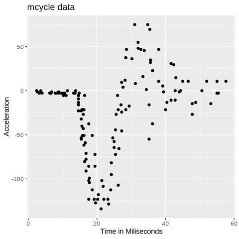
Figure 6.3: mcycle data in R
binned mean:
To fit binned mean model we use the base R function supsmu as follows:
mod_binned_R <- with(mcycle, supsmu(times, accel))

plot(mcycle$times, mcycle$accel, xlab = "Times", ylab = "Acceleration")

# add fit lines
lines(mod_binned_R)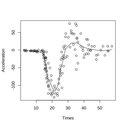
Figure 6.4: binned mean in R
local linear regression:
We use the base R function loess with different bandwidth values, say \(0.1\), \(0.3\), \(0.5\), \(0.75\)
# set the colors
cols<-c( "black", "green", "red", "blue")
spans=c(0.1, 0.3, 0.5, 0.75)
# plot the data points
plot(mcycle$times, mcycle$accel, xlab = "Times", ylab = "Acceleration")

for (i in 1:4){
  model <- with(mcycle, loess(accel~times, degree=1,span=spans[i]))
  lines(predict(model), x=mcycle$times, lwd = i, lty = i, col = cols[i])
}
legend("bottomright", c("span=0.1", "span=0.3", "span=0.5", "span=0.75"),
       lwd = 1:4, lty = 1:4, col = c( "black", "green", "red", "blue"), bty = "n")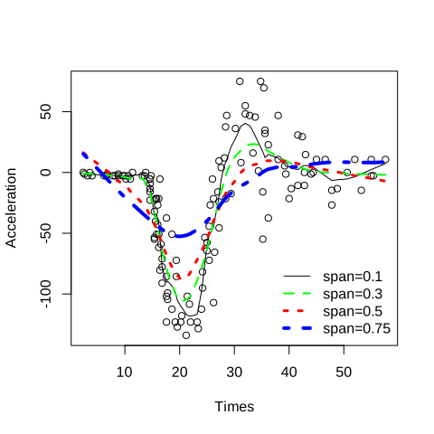
Figure 6.5: local linear rgression in R
As we see, small values for the bandwidth lead to more flexible model.
local polynomial regression:
Unfortunately, the loess function can fit a local polynomial regression up to second order. So in order to fit higher order we will use the R package KernSmoot
library(KernSmooth)
# set the colors
cols<-c( "black", "red", "blue")
polys<-c(2, 3, 4)

# plot the data points
plot(mcycle$times, mcycle$accel, xlab = "Times", ylab = "Acceleration")

for (i in 1:3){
  model <- with(mcycle, locpoly(times, accel, degree=polys[i], bandwidth=0.5))
  lines(model, lwd=i, lty = i, col = cols[i])
}
legend("bottomright", c("deg=2", "deg=3", "deg=4"),
        lwd=i,lty = 1:4, col = c( "black", "red", "blue"), bty = "n")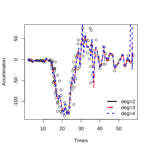
Figure 6.6: local polinomial rgression in R
Local constant regression:
Again we will use the same above package KernSmoot. For the kernels, we will use the Gaussian and the Epanechnikove distributions:
# set the colors
cols<-c("red", "blue")
kernels=c("normal", "epanech")

# plot the data points
plot(mcycle$times, mcycle$accel, xlab = "Times", ylab = "Acceleration")

for (i in 1:2){
  model <- with(mcycle, locpoly(times, accel, kernel=kernels[i], degree=0, bandwidth=0.5))
  lines(model, lwd=i, lty = i, col = cols[i])
}
legend("bottomright", c("normal", "epanech"),
        lwd=i,lty = 1:4, col = cols, bty = "n")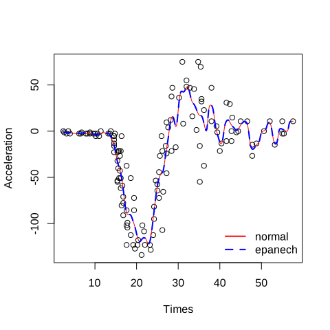
Figure 6.7: local constant rgression in R
Since we do not have a large sample size (\(n=133\)), the two kernels are almost the same.
Splines:
To apply this regression in R, we should call the R package splines2 and use the function bSpline. By inspecting the data, we should use three knots, \(15\), \(23\), and \(35\). However, the orders used in polynomial regression are the second and the third order.
To apply this regression in R, we should call the R package splines2 and use the function bSpline. By inspecting the data, we should use three knots, 1515, 2323, and 3535.
library(splines2)
# the default degree is 3
model <- with(mcycle, lm(accel ~ bSpline(times,knots = c(15,23,35))))
model2 <- with(mcycle, lm(accel ~ bSpline(times,knots = c(15,23,35), degree = 2)))

plot(mcycle$times, mcycle$accel, xlab = "Times", ylab = "Acceleration")
lines(mcycle$times, predict(model), col = "red", lty=1)
lines(mcycle$times, predict(model2), col = "green", lty=2)

#adding knots
abline(v=c(15,23,35),lty=2,col="darkblue")
legend("bottomright", c("deg=3", "deg=2"),
        lty = 1:2, col = c( "red", "green"), bty = "n")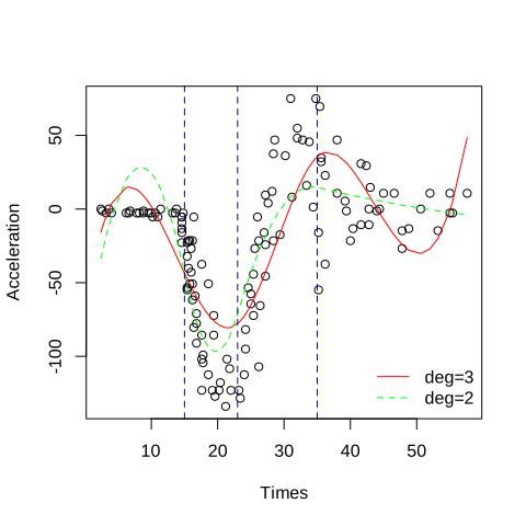
Figure 6.8: splines in R
As always, We first move the data to python
To perform non parametric regressions in python, we will use the package statsmodels
Local Constant regression
from statsmodels.nonparametric.kernel_regression import KernelReg
import numpy as np
import matplotlib.pyplot as plt

#to get the local constant we set reg_type to lc
# the bandwidth value in bw
# we have also to set the variable types in var_type, c for continuous

mod_lc_py = KernelReg(endog=mcycle_py.accel, exog=mcycle_py.times, reg_type='lc', bw=np.array([0.3]), var_type='c', ckertype='gaussian').fit()

# plot the result
fig= plt.figure(figsize=(5,3))
plt.plot(mcycle_py.times, mcycle_py.accel, 'o', alpha=0.5)
plt.plot(mcycle_py.times, mod_lc_py[0], 'r--' )
plt.savefig('mod_lc_py.png')
plt.clf()
plt.close()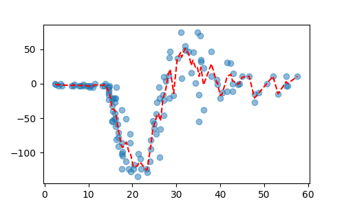
Figure 6.9: Local Constant regression in Python
Local linear regression:
We will use the same above code, except here we change th reg_type from lc to ll:
#to get the local linear we set reg_type to ll
mod_ll_py = KernelReg(endog=mcycle_py.accel, exog=mcycle_py.times, reg_type='ll', bw=np.array([0.3]), var_type='c', ckertype='gaussian').fit()

# plot the result
fig= plt.figure(figsize=(5,3))
plt.plot(mcycle_py.times, mcycle_py.accel, 'o', alpha=0.5)
plt.plot(mcycle_py.times, mod_ll_py[0], 'r--' )
plt.savefig('mod_ll_py.png')
plt.clf()
plt.close()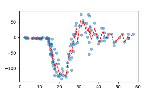
Figure 6.10: Local Linear regression in Python
Local Polynomial Regression:
For higher polynomial orders, we will use the package localreg:
from localreg import *
# we use the epanechnikov kernel and 0.3 for the bandwidth
y1 = localreg(mcycle_py.times.values, mcycle_py.accel.values, degree=2, kernel=rbf.epanechnikov, frac=0.3)
y2 = localreg(mcycle_py.times.values, mcycle_py.accel.values, degree=3, kernel=rbf.epanechnikov, frac=0.3)
y3 = localreg(mcycle_py.times.values, mcycle_py.accel.values, degree=4, kernel=rbf.epanechnikov, frac=0.3)
fig= plt.figure(figsize=(5,3))
plt.plot(mcycle_py.times, mcycle_py.accel, 'o', alpha=0.5)
plt.plot(mcycle_py.times, y1, color='black', label='deg=2')
plt.plot(mcycle_py.times, y2, color='red', label='deg=3')
plt.plot(mcycle_py.times, y3,color='blue', label='deg=4')
plt.legend()
plt.savefig('mod_poly_py.png')
plt.clf()
plt.close()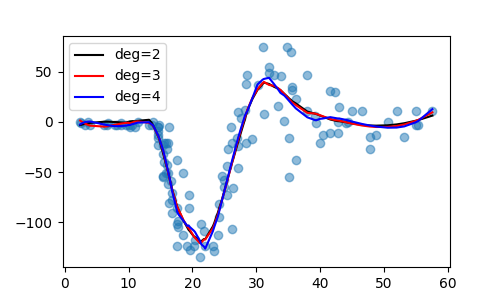
Figure 6.11: Local polynomial regression in Python
Splines
To fit regression with splines, we will use the basis function bs in the dmatrix module from the patsy package.
from patsy import dmatrix
import statsmodels.api as sm
import statsmodels.formula.api as smf

# create the splines with second order polynomial
x_basis2=dmatrix("bs(times, knots=(15,23,35), degree=2, include_intercept=False)", {"times": mcycle_py.times.values},return_type='dataframe')

# Cubic splines
x_basis3=dmatrix("bs(times, knots=(15,23,35), degree=3, include_intercept=False)", {"times": mcycle_py.times.values},return_type='dataframe')

# dmatrix returns a 0-based RangeIndex, while a data frame coming from R via
# reticulate is 1-based. statsmodels now requires endog/exog indices to match.
x_basis2.index = mcycle_py.index
x_basis3.index = mcycle_py.index

# fit generalized models
mod_splin_py2=sm.GLM(mcycle_py.accel, x_basis2).fit()
mod_splin_py3=sm.GLM(mcycle_py.accel, x_basis3).fit()

# plot the results
fig= plt.figure(figsize=(5,3))
plt.plot(mcycle_py.times, mcycle_py.accel, 'o', alpha=0.5)
plt.plot(mcycle_py.times, mod_splin_py2.fittedvalues,'g--', label='deg=2')
plt.plot(mcycle_py.times, mod_splin_py3.fittedvalues, color='r', label='deg=3')
plt.legend()
plt.savefig('mod_spline_py.png')
plt.clf()
plt.close()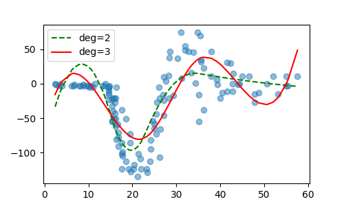
Figure 6.12: Splines in Python