5.2 Heteroskedasticity
We say that the disturbances \(\varepsilon_t\) are heteroskedastic if they have different variance values \(Var(\varepsilon_t)=\sigma^2_t\not=\sigma^2\) ( At least two of which are different). Violating, therefore, assumption 3 of homoskedasticity. The following exhibit shows examples of data affected by heteroskedasticity in which the scatter points indicate some pattern. It can be either linear or not, increases or decreases across observations or over time (in time series). That does not mean that under heteroskedasticity, the error variances must be all different from each other. It can exist sum subsets or groups of errors with the same variance but different from the other ones. In the exhibit below, the variances seem to increase over time.
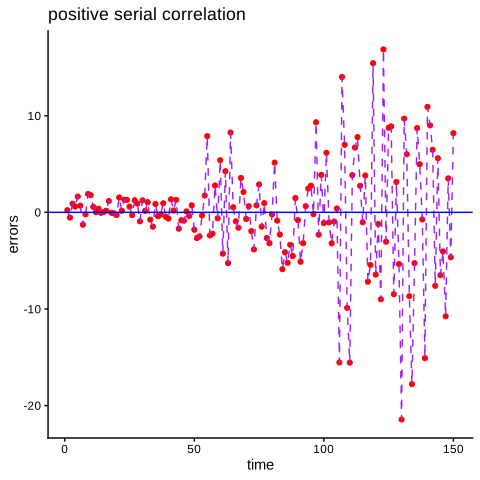
Figure 5.6: pattern of heteroskedasticity
In many applications, we can not sample data from a particular population without being affected by heteroskedasticity. The cross-sectional data are more likely to be affected than time series. For instance, if we have to consider a model in which the household income is supposed to explain the spending on a particular good. Consequently, we expect that the variations among families with high income will be higher (since they have more choices between expensive and cheaper goods) than those among families with low income (with fewer choices). Hence heteroskedasticity will be unavoidable.
For ease of investigation, we suppose that all the classical assumptions including autocorrelation are satisfied except that of homoskedasticity. Formally, let us consider our original model \(y=X\beta+\varepsilon\), the variance matrix of the disturbances under heteroskedasticity could be:
\[\begin{equation} \Omega_{\varepsilon}= \begin{pmatrix} \sigma^2_1&0&0&..&0\\ 0&\sigma^2_2&0&..&0\\ ..&..&..&..&..&\\ 0&0&0&0&\sigma^2_n \end{pmatrix} \tag{5.27} \end{equation}\]
Which is a diagonal matrix since the elements of the off diagonal are equal to zero. This is due to the non autocorrelation. For simplification, we can rewrite that matrix as follows:
\[\begin{equation} \Omega_{\varepsilon}=\sigma^2 \begin{pmatrix} \omega_1&0&0&..&0\\ 0&\omega_2&0&..&0\\ ..&..&..&..&..&\\ 0&0&0&0&\omega_n \end{pmatrix}=\sigma^2\Omega \tag{5.28} \end{equation}\]
Where the constant term \(\sigma^2=\frac{\sum\limits^{n}_{i=1}\sigma^2_i}{n}\) is the average of the diagonal elements of the matrix (5.27), and the elements of the matrix \(\Omega\) then are \(\omega_i=\frac{\sigma^2_i}{\sigma^2}\). With that transformation, the trace of the matrix \(\Omega\) will be \(tr(\Omega)=\sum\limits^{n}_{i=1}\omega_i=n\). This result will be useful further.
5.2.1 The OLS properties under hetroskedasticity
We will first verify the unbiasedness. With fixed regressors, we have:
\[\begin{align*} E\big(\widehat\beta\big)&=E\bigg[\big(X^tX\big)^{-1}X^ty\bigg] \\ &=\beta+\bigg(X^tX\bigg)^{-1}X^t\overbrace{E\big(\varepsilon\big)}^{=0} \\ &=\beta \end{align*}\]
And with stochastic regressors, we have:
\[\begin{equation*} E\big(\widehat\beta\big)=\beta+\overbrace{plim\bigg(\frac{1}{n}X^tX\bigg)^{-1}}^{=Q^{-1}}\overbrace{plim\bigg(\frac{1}{n}X^t\varepsilon\bigg)}^{=0}=\beta \end{equation*}\]
As with autocorrelation, unbiasedness and consistency are not affected.
However, the variance matrix will be:
\[\begin{align} Var\big(\widehat\beta\big)&=E\bigg[\big(\widehat\beta-\beta\big)\big(\widehat\beta-\beta\big)^t\bigg] \notag \\ &=E\bigg[\big(X^tX\big)^{-1}X^t\varepsilon\varepsilon^tX\big(X^tX\big)^{-1}\bigg] \notag \\ &=\big(X^tX\big)^{-1}X^t\overbrace{E\big(\varepsilon\varepsilon^t\big)}^{=\sigma^2\Omega}X\big(X^tX\big)^{-1} \notag \\ &=\sigma^2\big(X^tX\big)^{-1}\big(X^t\Omega X\big)\big(X^tX\big)^{-1} \tag{5.29} \end{align}\]
Since \(\sigma^2\Omega\not=\sigma^2\), this variance matrix does not equal to the classical one \(Var\big(\widehat\beta\big)=\sigma^2\big(X^tX\big)^{-1}\). The variance computed from (5.29) is not minimum, because the minimum one is in (5.20) computed with GLS method.
If we consider, for instance, the simple linear model (with demeaned variables for simplification) under heteroskedasticity \(E(\varepsilon_i)=\sigma^2_i\). The OLS estimator will still the same:
\[\begin{equation*} \widehat\beta=\frac{\sum x_iy_i}{\sum x^2_i} \end{equation*}\]
Its variance, in contrast, will be:
\[\begin{align*} Var\big(\widehat\beta\big)&=E\big(\widehat\beta-\beta\big)^2 \\ &=E\Bigg(\frac{\sum\limits_i x_i\varepsilon_i}{\sum\limits_i x^2_i}\Bigg)^2 \\ &=\frac{\sum\limits_i x^2_iE\big(\varepsilon_i\big)^2}{\big(\sum \limits_i x^2_i\big)^2} \\ &=\frac{\sum \limits_i x^2_i\sigma_i^2}{\big(\sum \limits_i x^2_i\big)^2}\\ &\not=\frac{\sigma^2}{\sum \limits_i x^2_i} \end{align*}\]
That means that if, under heteroskedasticity, we continue to use the classical variance, the associated statistic test such as t-test will give misleading results.
Even the OLS estimators are not efficient, they maintain the asymptotic normality distribution. This can be proved, without much detail, by using the central limit theorem. Under some suitable conditions (Green 2018), we will have:
\[\begin{equation} \sqrt{n}\big(\widehat\beta-\beta\big)=\Bigg(\frac{1}{n}X^tX\Bigg)^{-1}\frac{1}{\sqrt{n}}X^t\varepsilon \tag{5.30} \end{equation}\]
The variance of the last term of the right hand side \(\frac{1}{\sqrt{n}}X^t\varepsilon\) is:
\[\begin{align} Var\bigg(\frac{1}{\sqrt{n}}X^t\varepsilon\bigg)&= \frac{1}{\sqrt{n}}X^tE\big(\varepsilon\varepsilon^t\big)X\frac{1}{\sqrt{n}} \notag \\ &= \sigma^2\bigg(\frac{1}{n}X^t\Omega X\bigg) \tag{5.31} \end{align}\]
Assuming that \(plim\Bigg(\frac{1}{n}X^tX\Bigg)=Q\) and \(plim\bigg(\frac{1}{n}X^t\Omega X\bigg)=Q_{\Omega}\) are both finite positive definite matrices, and using the expression (5.31), the asymptotic variance of \(\widehat\beta\) will be:
\[\begin{equation} Var_{Asy}\big(\widehat\beta\big)=\frac{\sigma^2}{n}Q^{-1}Q_{\Omega}Q^{-1} \tag{5.32} \end{equation}\]
That is:
\[\begin{equation} \widehat\beta\approx \mathrm N\Bigg(\beta,\frac{\sigma^2}{n}Q^{-1}Q_{\Omega}Q^{-1}\Bigg) \tag{5.33} \end{equation}\]
5.2.2 Causes of heteroskedasticity
It is critical to distinguish between heteroskedasticity caused by misspecification of the model (such as omitting relevant variables) and that caused by the data, even if the model is correctly specified. In the former case, the problem is more serious than heteroskedasticity (see 3.8) because the model is wrong, and we should fix this problem first. However, The second case is what we will discuss in this subsection. That is, we expect everything is fine except for the heteroskedasticity assumption.
Practitioners have listed the following reasons behind this problem:
- If the data samples are collected from a population characterized by higher variances for errors related to larger observation values and small ones related to the smaller ones. That is why, heteroskedasticity is more likely to occur in cross-sectional data than time series.
- Some time series can give arise of heteroskedasticity. For instance, a beginner in driving learning, his mistakes decrease as time increases. Thus, the observation variances become smaller than they were before. Models with this type of behavior called Error learning models.
- if the data are collected as averages. For instance, the average wages in each firm. The disparity therefore increases as long as the firm profits increases.
- Presence of large number of outliers in the data cab give rise of heteroskedasticity, especially in small samples.
5.2.3 Testing for heteroskedasticity
Visual inspection is the first step to check heteroskedasticity. For instance, we can represent the squared residuals of the estimated model \(e_i^2\) in graph. Since by intuition the natural estimator of \(\sigma^2_i\), where the squared residuals in the vertical axis and the fitted values in the horizontal axis. If we detect a certain pattern then heteroskedasticity is more likely to be present. The squared residuals can also be plotted against one of the model regressors if this regressor is suspected to be the source of the problem.
Example 5.2 To well understand this subject, we will simulate heteroskedastic data. we will thus create three group of errors with different variances using the poisson distribution via one of the DGP regressors.
set.seed(4)

x3 <- c(rpois(100, 20), rpois(100, 60), rpois(100, 90))
e <- sapply(x3, function(i) rnorm(1, 0, sqrt(i)))
x2 <- rnorm(300, 3, 2)
y <- 1.2+0.7*x2+0.4*x3+e

data <- tibble(y=y, x2=x2, x3=x3)
mod_heter <- lm(y~x2+x3, data)
sqrd_error <- mod_heter$residuals**2
fitted <- mod_heter$fitted.values
df <- tibble(fitted=fitted, x3=x3, sqrd_error=sqrd_error)
g1 <- ggplot(df, aes(fitted, sqrd_error))+
  geom_point(color="red", size=1)+
  geom_smooth(method="loess", lty=2, color="purple")+
  labs(title="Squared errors against fitted values",
       y="Squared errors",
       x="Fitted values")+
  theme_classic()

g2 <- ggplot(df, aes(x3, sqrd_error))+
  geom_point(color="red", size=1)+
  geom_smooth(method="loess", lty=2, color="purple")+
  labs(title="Squared errors against the regressor x3",
       y="Squared errors",
       x="x3")+
  theme_classic()

g1 / g2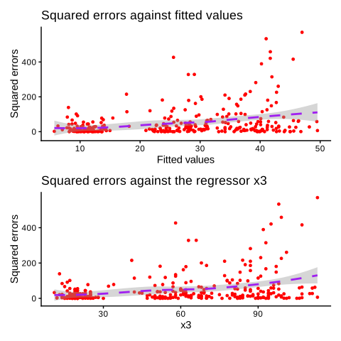
Figure 5.7: plots of heteroskedasticity
We see that in both plots, the squared errors increase with the increase of the corresponding variables (fitted values and \(x3\))
The drawback of the graphical methods is that, in most cases, we do not have a clear cut whether heteroskedasticity is present or not. Hence any decision will be based only on the personal judgment of each investigator. Therefore, formal statistic tests are needed to decide about this issue.
We should point out that all the tests discussed shortly are based on the assumption that the error variance can be explained by a function of other variables related somehow to the model at hand. That is \(\sigma^2_i=\mathrm g\big(z_{1i},z_{2i},..,z_{pi}\big)\). Researchers, by experience, recommend using the original regressors suspected to be the source of heteroskedasticity.
We should also note that the OLS estimator is BLUE if all the classical assumptions are satisfied. If we drop this estimator then in favor of another one assuming the presence of heteroskedasticity, but in fact, it is not, then the latter estimator is not efficient. In other words, we have to be sure about heteroskedasticity before looking for another alternative to the OLS estimator.
5.2.3.1 Park test
Introduced first by (Park 1966). The test is testing the following function:
\[\begin{equation*} \sigma^2_i=\sigma^2X_i^{\gamma}exp(v_i) \end{equation*}\]
This function can be linearized by including the natural logarithm:
\[\begin{equation} log\big(\sigma^2_i\big)=log\big(\sigma^2\big)+\gamma log\big(x_i\big)+v_i \tag{5.34} \end{equation}\]
Where \(x_i\) is the suspected regressor of being the original of the heteroskedasticity. To enable the estimation of that function, we should first replace the unknown \(\sigma^2\) by the squared residuals \(e_i^2\) (obtained from the estimation of the original model disregarding heteroskedasticity), and setting the constant term \(log\big(\sigma^2\big)=\alpha\), the above model than will be:
\[\begin{equation} log\big(e^2_i\big)=\alpha+\gamma log\big(x_i\big)+v_i \tag{5.35} \end{equation}\]
Then this final equation will be estimated by the classical method OLS. If the slop \(\gamma\) is significantly different from zero then the null hypothesis of homoskedasticity will be rejected in favor of heteroskedasticity. However, this test has been criticized because the errors \(v_i\) are more likely to be autocorrelated or heteroskedastic or both. In such cases, the t-test will no longer still reliable (Goldfeld and Quandt 1972).
If we are not sure about the regressor that should include in that function, we can use all of them one by one. Therefore, if all of the coefficients are insignificant, we can not reject the null hypothesis.
5.2.3.2 Glejser test
This test (Glejser 1969) differs from the previous one only in the suggested functional forms. To perform it Glesjer has suggested using the absolute values of the residuals against one of the regressors in six different structures, where two of which are non-linear in parameters:
\[\begin{align} &|e_i|=\alpha+\gamma x_i+v_i, \quad |e_i|=\alpha+\gamma \frac{1}{x_i}+v_i, \quad |e_i|=\sqrt{\alpha+\gamma x_i}+v_i \\ &|e_i|=\alpha+\gamma \sqrt{x_i}+v_i, \quad |e_i|=\alpha+\gamma \frac{1}{\sqrt{x_i}}+v_i, \quad |e_i|=\sqrt{\alpha+\gamma x^2_i}+v_i \tag{5.36} \end{align}\]
After running these regressions by OLS for the first four ones and NLS (non-linear least squares) for the rest, we check the significance of each \(\gamma\). If at least one of which is significant, then heteroskedasticity is present.
Such as the previous test, this one faces the same critics about the errors \(v_i\) being autocorrelated and heteroskedastic.
5.2.3.3 Goldfeld Quandt test
The idea behind this test is quite simple (Goldfeld and Quandt 1965). Order the observations according to the regressor \(x_i\) (suspected to be the source of heteroskedasticity), then split them into two sets. Consequently, each set now will have its error variance (\(\sigma^2_1\) for the first and \(\sigma^2_2\) for the second). The null hypothesis should be \(H0:\sigma^2_1=\sigma^2_2\) against \(H1:\sigma^2_1<\sigma^2_2\). Since these two variances are unknown, we can replace them with the estimated \(s_1^2\) and \(s_2^2\). Finally, we use the \(F-test\) to test if the two variances are significantly different or not. We can summarize the process of this test as follows:
- Rank the observations according to the suspected regressor.
- Remove some of the central observations, say \(c\) observations, that must be appropriately specified (the authors of the test suggest \(c=8\) for \(n=30\), and \(c=16\) for \(n=60\)). The remaining observations give two sets, each of which has \(\frac{n-c}{2}\) observations.
- Run OLS regression on each set and compute the associated sum of squared residuals \(e_1^te_1\) and \(e_2^te_2\), where each of which has \(\frac{n-c-2k}{2}\) degrees of freedom. Then compute the estimated variances \(s^2_1\) and \(s^2_2\).
- The ratio \(F^c=\frac{s_2^2\big/\sigma^2_2}{s_1^2\big/\sigma^2_1}\) follows the \(F\bigg(\frac{n-c-2k}{2},\frac{n-c-2k}{2}\bigg)\) distribution. Under the null hypothesis of homoskedasticity (with all the remaining classical assumptions) that ratio reduces to \(F^c=\frac{s_2^2}{s_1^2}\). Therefore, we reject the null hypothesis if the value of that ratio is higher than the critical one at the chosen significance level.
We have to notice that the power of this test depends, among others, on the specified value of \(C\), which decreases when that value increases.
5.2.3.4 LR test
The previous test can be extended to the data that may have several groups, where each of which has a constant variance but it is supposed to be different from the variances of the other groups. As a result, the null hypothesis now is \(H0:\sigma^1_2=\sigma^1_2=..=\sigma^2_\mathrm g\).
Let us denote the number of the observations of the group \(i\) by \(n_i\) such that \(n=\sum\limits^{\mathrm g}_{i=1}n_i\). Thus our original model \(y=X\beta+\varepsilon\) can be rewritten in terms of the observations of each group as follows:
\[\begin{align*} \begin{pmatrix}y_1\\y_2\\..\\y_\mathrm g\end{pmatrix}= \begin{pmatrix}X_1\\X_2\\..\\X_\mathrm g\end{pmatrix}\beta+ \begin{pmatrix}\varepsilon_1\\\varepsilon_2\\..\\\varepsilon_\mathrm g\end{pmatrix} \end{align*}\]
And the disturbances variance matrix under homoskedasticity is given by:
\[\begin{equation*} Var(\varepsilon)=\sigma^2I \end{equation*}\]
Whereas, under heteroskedasticity, it is given by::
\[\begin{equation} Var(\varepsilon)= \begin{pmatrix} \sigma^2_1I_{n_1}&0&0&..&0\\ 0&\sigma^2_2I_{n_2}&0&..&0\\ ..&..&..&..&..\\ 0&0&0&..&\sigma^2_{\mathrm g}I_{n_{\mathrm g}} \end{pmatrix}=\Omega_{\varepsilon}\not=\sigma^2 \tag{5.37} \end{equation}\]
To apply this test, we have to compute the maximum log likelihood under the null hypothesis, which is called the restricted maximum log likelihood (because the assumption of equality of the variances is considered as a restriction against the general situation where they are different) and the unrestricted maximum log likelihod under the alternative hypothesis of heteroskedasticity.
The former one therefore is expressed by:
\[\begin{equation} l_{restricted}=-\frac{n}{2}log\big(2\pi\big)-\frac{1}{2}log\big(\sigma^2\big)-\frac{1}{2\sigma^2}\big(y-X\beta\big)^t\big(y-X\beta\big) \tag{5.38} \end{equation}\]
By maximizing this function with respect to the parameters \(\beta\) and \(\sigma^2\), we get the classical estimator \(\beta_{ML}=\big(X^tX\big)^{-1}(X^ty\big)=\widehat\beta\) and \(\widehat\sigma^2=\frac{\big(y-X\widehat\beta\big)^t\big(y-X\widehat\beta\big)}{n}\). Substituting those estimates into (5.38) we get the value of \(l_{restricted}\).
Similarly, the unrestricted function will be:
\[\begin{equation} l_{unrestricted}=-\frac{n}{2}log\big(2\pi\big)-\frac{1}{2}log\big(det(\Omega_{\varepsilon})\big)-\frac{1}{2}\big(y-X\beta\big)^t\Omega^{-1}_{\varepsilon}\big(y-X\beta\big) \tag{5.39} \end{equation}\]
Or in terms of the the group variances:
\[\begin{equation} l_{unrestricted}=-\frac{n}{2}log\big(2\pi\big)-\frac{n_1}{2}log\big(\sigma_1^2\big)-..-\frac{n_{\mathrm g}}{2}log\big(\sigma_{\mathrm g}^2\big)-\frac{1}{2}\big(y-X\beta\big)^t\big(y-X\beta\big) \tag{5.40} \end{equation}\]
The estimator of \(\beta\) now is the GLS one \(\beta_{ML}=\big(X^t\Omega^{-1}_{\varepsilon}X\big)^{-1}X^t\Omega^{-1}_{\varepsilon}y=\beta_{GLS}\). Since, in general, \(\Omega_{\varepsilon}\) is unknown, we can use the FGLS discussed in the subsection (5.1.4.3) to get the estimates \(\beta_{GLS}=\big(X^t\widehat\Omega^{-1}_{\varepsilon}X\big)^{-1}X^t\widehat\Omega^{-1}_{\varepsilon}y\). Then compute the variance of each group using the following expression:
\[\begin{equation*} \widehat\sigma^2_i=\frac{1}{n_i}\bigg(y-X_i\beta_{GLS}\bigg)^t\bigg(y-X_i\beta_{GLS}\bigg) \end{equation*}\]
By plug in these estimates into the variance matrix (5.37), we get the estimated matrix \(\widehat\Omega_{\varepsilon}\), which will be used in turn to get \(\beta_{GLS}\). However, we can see that \(\widehat\Omega_{\varepsilon}\) and \(\beta_{GLS}\) depend on each other to be computed. To solve this problem, we can start by estimating each group separately by OLS method (since the variance within the group is constant so the estimators should be efficient) and compute each variance by \(\widehat\sigma^2_i=\frac{\bigg(y_i-X_i\widehat\beta_i\bigg)^t\bigg(y_i-X_i\widehat\beta_i\bigg)}{n_i}\). Then, using these variance values to get the estimated matrix and hence the regression coefficients, and finally, the value of \(l_{unrestricted}\).
At this step we are ready to compute the LR-test as follows:
\[\begin{equation} LR=2\big(l_{restricted}-l_{unrestricted}\big)\approx\chi_{(\mathrm g)}^2 \tag{5.41} \end{equation}\]
Larger value for this test reject the null hypothesis (\(H0:\) homoskedasticity).
Lastly, we have to notice that this test requires large samples to get the asymptotic normality for the maximum likelihood and allow performing the separate regression in each group.
5.2.3.5 Breush-Pagan-test BP-test
This test, developed by (S.Breusch and R.Pagan 1979). It assumes that the every observation variance is a linear function of some variables as follows:
\[\begin{equation} \sigma^2_i=\gamma_1+\gamma_2z_{2i}+..+\gamma_pz_{pi}+v_i \tag{5.42} \end{equation}\]
Where, \(v_i\) is assumed to be white noise. We can estimate that equation by, first, replacing \(\sigma^2_i\) by the estimated residuals \(e_i^2\), then applying the usual LM-test \(LM=nR^2\) (derived in the subsection (3.9.5)) that follows, under the null hypothesis, \(\chi^2_{(p-1)}\).
Larger values for this test lead to reject the null hypothesis. However, this test supposes that the variables \(z_i\) are known, which is not the case for the most applications.
5.2.3.6 White test
This test can be seen as a feasible version of the previous one, such that the variables \(z_i\) could be replaced by some function of the original regressors. The two most common forms are:
The first one is without cross product:
\[\begin{equation} e_i^2=\gamma_1+\gamma_2x_{2i}+..+\gamma_kx_{ki}+\gamma_{k+1}x_{2i}^2+..+\gamma_{2k-1}x_{ki}^2+v_i \tag{5.43} \end{equation}\]
Whereas, the second one is with cross product:
\[\begin{equation} e_i^2=\gamma_1+\gamma_2x_{2i}+..+\gamma_kx_{ki}+\gamma_{k+1}x_{2i}^2+..+\gamma_{2k-1}x_{ki}^2+..+\underset{0\leqslant s\leqslant \frac{(k-1)!}{2!(k-3)!}}{\gamma_{2k+s}}\underset{2\leqslant h < l \leqslant k}{x_{hi}x_{li}}+..+v_i \tag{5.44} \end{equation}\]
Then, applying the usual LM-test on these regressions. Note that the degrees of freedom of \(\chi^2\) for th first equation is \(p-1=2k-1-1=2k-2\), and for the second is \(p-1=2k+\frac{(k-1)!}{2!(k-3)!}-2\).
An interesting property of this test is that not only used to test heteroskedasticity but also for testing misspecification. Therefore, we have to be cautious in interpreting this test.
5.2.3.7 Spearman’s rank correlation test
The well known correlation coefficient for qualitative variables is called Spearman’s rank correlation test. It is given by:
\[\begin{equation} r_s=1-6\Bigg(\frac{\sum d_i}{n(n^2-1)}\Bigg) \tag{5.45} \end{equation}\]
Where \(d_i\) is the difference in the rank for the \(i^{th}\) individual.
To be computed, this coefficient requires both variables be ordered. For heteroskedasticity, this coefficient can be used to detect any correlation between the absolute values of the model residuals and one of the regressors \(x_i\) (or the fitted values \(\widehat y_i\)). The derived test for testing the significance of this coefficient thus can be defined by:
\[\begin{equation} t^c=\frac{r_s\sqrt{n-2}}{\sqrt{1-r_s^2}} \tag{5.46} \end{equation}\]
It follows the t-student with \(n-2\) degrees of freedom.
Larger values lead to reject the null hypothesis.
Let us use the data gnerated in 5.2.
First we fit the OLS model:
Park test:
To apply this test we fit the function (5.35) using the resulted residuals from the above model mod_hetero.
mod_park <- lm(loge_sq~logx3, data=tibble(loge_sq=log(mod_hetero$residuals**2), logx3=log(x3)))
tidy(mod_park)
[out] # A tibble: 2 × 5
[out] term estimate std.error statistic p.value
[out] <chr> <dbl> <dbl> <dbl> <dbl>
[out] 1 (Intercept) -0.959 0.714 -1.34 0.180
[out] 2 logx3 0.912 0.183 4.99 0.00000101Since \(\gamma\) is highly significant (p-value is much smaller than the threshold of \(0.05\)), we reject the null hypothesis of homoskedasticity. That is we have heteroskedastic problem.
Glejser test:
There exists an R package dedicated for heteroskedasticity that has a lot of tests in addition to those discussed in this book called skedastic.
[out] # A tibble: 1 × 4
[out]   statistic       p.value parameter alternative
[out]       <dbl>         <dbl>     <dbl> <chr>
[out] 1      39.0 0.00000000335         2 greater
Since the p-value is very small, we will reject the null hypothesis of homoskedasticity.
Goldfeld Quandt test:
[out] # A tibble: 1 × 5
[out]   statistic  p.value parameter method                 alternative
[out]       <dbl>    <dbl>     <int> <chr>                  <chr>
[out] 1      4.22 5.31e-12        97 Goldfeld-Quandt F Test greater
This test also has detected heteroskedasticity.
Breush-Pagan-test:
[out] # A tibble: 1 × 5
[out]   statistic     p.value parameter method                alternative
[out]       <dbl>       <dbl>     <dbl> <chr>                 <chr>
[out] 1      31.1 0.000000180         2 Koenker (studentised) greater
As expected this test also has detected heteroskedasticity.
White test:
[out] # A tibble: 1 × 5
[out]   statistic     p.value parameter method       alternative
[out]       <dbl>       <dbl>     <dbl> <chr>        <chr>
[out] 1 34.3 0.000000656 4 White's Test greaterFirst let us move the data from R to python.
Park test:
We will do the same as we did in R. We fit the OLS model using the equation (5.35) as follows:
df_park = pd.DataFrame({"log_sq":np.log(mod_hetero_py.resid**2), "logx3":np.log(data_hetero_py.x3)})[out] Coef. Std.Err. t P>|t| [0.025 0.975]
[out] Intercept -0.959443 0.714115 -1.343542 0.180119 -2.364790 0.445904
[out] logx3 0.911730 0.182565 4.993993 0.000001 0.552449 1.271011The variable logx3 is highly significant, so we have heteroskedasticity problem.
Glejser test:
This test does not exist in statsmodels package. We will thus implement this test by hand. But for simplification we will use only the first four equations in (5.36) (since we will find at least one significant relationship).
import statsmodels.api as sm

df_glesjer = pd.DataFrame()
df_glesjer["error"] = np.abs(mod_hetero_py.resid)
df_glesjer["z1"]=data_hetero_py[["x3"]]
df_glesjer["z2"]=np.sqrt(data_hetero_py[["x3"]])
df_glesjer["z3"]=np.reciprocal(data_hetero_py[["x3"]].astype("float"))
df_glesjer["z4"]=np.reciprocal(np.sqrt(data_hetero_py[["x3"]]))


pvalues=[]
y=df_glesjer["error"]

for i in df_glesjer.columns[1:]:
  x=df_glesjer[i]
  mod_glesjr=smf.ols("y~x", df_glesjer).fit()
  pvalues.append(mod_glesjr.pvalues[1])

# display only the p-values of the slopes
pvalues
[out] [2.666013351375056e-09, 3.820787272284662e-09, 2.5249008543355524e-07, 4.252182044959226e-08]We see that all the p-values have small values so that the null hypothesis should be rejected.
Goldfeld Quandt test:
import statsmodels.stats.api as sms
from statsmodels.compat import lzip
name = ['F statistic', 'p-value']

# idx defines the index of the column that should be used to sort the data
# 2 refers to x3
GQ = sms.het_goldfeldquandt(mod_hetero_py.resid, mod_hetero_py.model.exog, idx=2)
lzip(name, GQ)
[out] [('F statistic', 2.6475307772740773), ('p-value', 3.692638994621356e-09)]Breush-Pagan-test:
keys = ['LM statistic:', 'LM p-value:', 'F-test:', 'F-test p-value:']
BP = sms.het_breuschpagan(mod_hetero_py.resid,mod_hetero_py.model.exog )
lzip(keys, BP)
[out] [('LM statistic:', 31.061302754045883), ('LM p-value:', 1.7993838017562427e-07), ('F-test:', 17.151133348271646), ('F-test p-value:', 8.933224507097441e-08)]White test:
keys = ['LM statistic:', 'LM p-value:', 'F-test:', 'F-test p-value:']
WH = sms.het_white(mod_hetero_py.resid,mod_hetero_py.model.exog )
lzip(keys, WH)
[out] [('LM statistic:', 35.92400653256003), ('LM p-value:', 9.836409720918065e-07), ('F-test:', 7.998953469335241), ('F-test p-value:', 4.360231368664663e-07)]5.2.4 Estimation under heteroskedasticity
We showed in the preceding analysis that the OLS estimators still consistent but not efficient. We introduced also another consistent and efficient estimators based on the GLS method. The big issue with this method is that the matrix \(\Omega_{\varepsilon}\) rarely when all of its elements are known. That is why a variety of methods exist to estimate that matrix. In the following subsections, we will discuss the most popular ones.
5.2.4.1 Weighted least squares WLS
If we consider the matrix \(\Omega^{-1}_{\varepsilon}\) as a weighting matrix in the GLS formula \(\beta_{GLS}=\big(X^t\Omega^{-1}_{\varepsilon}X\big)^{-1}X^t\Omega^{-1}_{\varepsilon}y\), then the GLS estimator can be also called Weighted least squares estimators. Analogously, the OLS estimators can also be seen as weighted estimators with the identity matrix \(I\) as weighting matrix \(\widehat\beta=\big(X^tI^{-1}X\big)^{-1}X^tI^{-1}y\), called also unweighted least squares or equally weighted least squares.
The idea behind this method is merely to give more importance to observations that have smaller variances and less importance to those with larger variances. The least squares criterion thus will be (in case of the simple linear regression):
\[\begin{equation} S=Min\sum\limits_iw_i\big(y_i-\alpha-\beta x_i\big)^2 \tag{5.47} \end{equation}\]
Where \(w_i\) should increase if \(\sigma_i^2\) decreases. The simple representation is when the former variable is equal to the inverse of the latter one as follows:
\[\begin{equation} S=Min\sum\limits_i\frac{\big(y_i-\alpha-\beta x_i\big)^2}{\sigma^2_i} \tag{5.48} \end{equation}\]
We can obtain the DGP model related to the last criterion by the following:
\[\begin{equation*} \frac{y_i}{\sigma_i^2}=\alpha\frac{1}{\sigma_i^2}+\beta \frac{x_i}{\sigma_i^2}+\frac{\varepsilon}{\sigma_i^2} \end{equation*}\]
where the error term \(\frac{\varepsilon}{\sigma_i^2}\) is homoskedastic:
\[\begin{equation*} E\Bigg(\frac{\varepsilon_i}{\sigma_i^2}\Bigg)^2=\frac{E\big(\varepsilon_i^2\big)}{\sigma_i^2}=\frac{\sigma_i^2}{\sigma_i^2}=1 \end{equation*}\]
Estimating therefore this model by OLS will give the same estimate such as the GLS one applied on the heteroskedastic model.
It should be noted that this model does not contain a constant term (since \(\frac{1}{\sigma_i^2}\) can also be considered as a variable), which means that we should be careful when interpreting the determination coefficient \(R^2\) since now is not bounded between 1 and 0 as usual.
For the generalized linear model, we have shown before that the GLS estimator is BLUE under heteroskedasticity and autocorrelation. Consequently, if the errors are still assumed uncorrelated, then by using the expression (5.28), the GLS estimator will be simplified to:
\[\begin{align} \beta_{GLS}&=\Bigg(\sum\limits_i\frac{1}{\omega_i}x_ix_i^t\Bigg)^{-1}\Bigg(\sum\limits_i\frac{1}{\omega_i}x_iy_i^t\Bigg) \notag \\ &=\Bigg(\sum\limits_iw_ix_ix_i^t\Bigg)^{-1}\Bigg(\sum\limits_iw_ix_iy_i^t\Bigg) \tag{5.49} \end{align}\]
Where \(w_i=\frac{1}{\omega_i}=\frac{\sigma^2}{\sigma^2_i}\). That is \(w_i\) is inversely proportional to \(\sigma^2_i\).
And the GLS variance matrix will be:
\[\begin{align} Var\big(\beta_{GLS}\big)&=\bigg(X^t\Omega_{\varepsilon}^{-1}X\bigg)^{-1} \notag \\ &=\Bigg(\sum\limits_i\frac{1}{\sigma_i^2}x_ix_i^t\Bigg)^{-1} \notag \\ &=\sigma^2\Bigg(\sum\limits_i\frac{1}{\omega_i}x_ix_i^t\Bigg)^{-1} \notag \\ &=\sigma^2\Bigg(\sum\limits_i w_ix_ix_i^t\Bigg)^{-1} \tag{5.50} \end{align}\]
Now if all the elements of this matrix \(\sigma_i^2\) (or \(\omega_i\)) are known, the computation of the estimates and their standard errors is straightforward and th problem of heteroskedasticity is solved. However, since the most applications they are not, so they should be estimated. Note that when \(\sigma_i^2\), the \(\sigma^2\) need not to be estimated which is just a scale factor that can be deduced by the following constraint:
\[\begin{align*} Tr\big(\Omega\big)=n \quad &\implies \quad \sum\limits_i\omega_i=\sum\limits_i \frac{\sigma_i^2}{\sigma^2} \\ &\implies \quad \sigma^2=\sum\limits_i \frac{\sigma_i^2}{n} \end{align*}\]
If the investigator can not determine the correct causes of heteroskedasticity, they can still use the OLS estimators but should correct the classical standard errors using the OLS residuals. Those new standard errors are called White’s heteroskedasticity consistent standard errors HAC.
One can suggest merely using the squared residuals \(e_i^2\) as an estimator of \(\sigma^2_i\). However, this estimator is not consistent because the estimation of each \(\sigma^2_i\) has just one single observation \(e_i^2\) even when the sample size is very large. But what about unbiasedness?
Let us express each single residual \(e_i\) in terms of the whole vector \(e\) as follows:
\[\begin{equation*} e_i=\underset{(1\times n)}{\begin{pmatrix}0&..&\overset{i^{th}}{1}&..&0\end{pmatrix}} \underset{(n\times 1)}{\begin{pmatrix}..\\e_i\\..\end{pmatrix}} \end{equation*}\]
Since \(e=M\varepsilon\) (where \(M=I-X\big(X^tX\big)^{-1}X^t\)), then each singla residual will be \(e_i=h_iM\varepsilon\), and Ones squared, it will be:
\[\begin{equation*} e_i^2=h_iM\varepsilon\varepsilon^tMh_i^t \end{equation*}\]
Hence:
\[\begin{align*} E\big(e_i^2\big)&=h_iME\big(\varepsilon\varepsilon^t\big)Mh^t_i \\ &= h_iM\Omega_{\varepsilon}Mh^t_i \\ &= \begin{pmatrix}0&..&1&..&0\end{pmatrix} \begin{pmatrix}..&..&..\\..&m_{kl}&..\\..&..&..\end{pmatrix} \begin{pmatrix}\sigma_1^2&0&0&..&0\\0&..&0&..&0\\0&0&\sigma_i^2&..&0\\..&..&..&..&..\\0&0&0&..&\sigma_n^2\end{pmatrix}\begin{pmatrix}..&..&..\\..&m_{kl}&..\\..&..&..\end{pmatrix}\begin{pmatrix}0\\..\\1\\..\\0\end{pmatrix}\\ &=\begin{pmatrix}m_{i1}&..&m_{in}\end{pmatrix}\begin{pmatrix}\sigma_1^2&0&0&..&0\\0&..&0&..&0\\0&0&\sigma_i^2&..&0\\..&..&..&..&..\\0&0&0&..&\sigma_n^2\end{pmatrix}\begin{pmatrix}m_{i1}\\..\\\\..\\m_{ik}\end{pmatrix}\\ &=m_{i1}^2\sigma_1^2+..+m_{ii}^2\sigma_i^2+m_{in}^2\sigma_n^2 \\ &\not=\sigma^2_i \end{align*}\]
Which means that \(e_i^2\) neither consistent nor unbiased estimator of \(\sigma_i^2\).
Sometimes, it may happen that \(\sigma_i^2\) can be partially known so that it can be approximated by a function of some known variables (some of which could be a subset or the whole set of the original regressors), say:
\[\begin{equation} \sigma_i^2=h\big(z_i^t\alpha\big) \tag{5.51} \end{equation}\]
However, even when the variables \(z_i\) and the function are correctly defined, the parameters \(\alpha\) rarely when they are known. Therefore, we must first estimate these parameters and then use their estimates to compute WLS estimates. This approach called two step weighted least squares or feasible weighted least squares FWLS. Those estimators are:
\[\begin{align} \beta_{FGLS}&=\Bigg(\sum\limits_i\frac{1}{\widehat\sigma^2_i}x_ix^t_i\Bigg)^{-1}\Bigg(\sum\limits_i\frac{1}{\widehat\sigma^2_i}x_iy^t_i\Bigg) \\ &=\Bigg(\sum\limits_i\frac{1}{h\big(z^t_i\widehat\alpha\big)}x_ix^t_i\Bigg)^{-1}\Bigg(\sum\limits_i\frac{1}{h\big(z^t_i\widehat\alpha\big)}x_iy^t_i\Bigg) \tag{5.52} \end{align}\]
For the estimation of \(\alpha\), we can reformulate the assumption \(E\big(\varepsilon_i^2\big)=\sigma_i^2\) (or \(E\big(\varepsilon_i^2/X\big)=\sigma_i^2\) in case of stochastic regressors) as follows:
\[\begin{equation} \varepsilon^2_i=\sigma^2_i+v_i \tag{5.53} \end{equation}\]
Where \(v_i\) is assumed to be a white noise.
But since \(\varepsilon^2_i\) is unknown, it can be replaced by \(e_i^2\). Then by using \(e^te=\varepsilon^tM\varepsilon\), the single residual can be expressed by \(e_i=\varepsilon_i-x_i^t\big(X^tX\big)^{-1}X^t\varepsilon\), The squared residuals will be expressed by:
\[\begin{equation*} e_i^2=\varepsilon^2_i-2\overbrace{\varepsilon_ix^t_i\big(X^tX\big)^{-1}X^t\varepsilon}^{u_i}+\overbrace{\bigg[x^t_i\big(X^tX\big)^{-1}X^t\varepsilon\bigg]^2}^{\eta_i} \end{equation*}\]
Substituting then (5.51) and (5.53) into the last expression, we obtain:
\[\begin{equation*} e_i^2=h\big(z^t_i\alpha\big)+v_i-2u_i+\eta_i \end{equation*}\]
We see that \(E(u_i)\not=0\) and \(E(\eta_i)\not=0\), but in large samples the lase two terms in the right hand side could be neglected. Assuming that \(h\) is a linear function (which is satisfied in most cases), the last expression reduces to the following:
\[\begin{equation*} e_i^2=z^t_i\alpha+\nu_i \end{equation*}\]
Therefore, the OLS applied on this equation gives consistent estimators \(\widehat\alpha\).
- There exists another alternative for replacing \(\sigma^2_i\) by \(\frac{e_i^2}{1-h_i}\), instead of \(e_i^2\), as a dependent variable in (5.53). This is because when we use \(e^te=\varepsilon^tM\varepsilon=\varepsilon^t\varepsilon-\varepsilon^tH\varepsilon\) (where \(H=X\big(X^tX\big)^{-1}X^t\)), the expectation of each single squared error is given by:
\[\begin{equation*} E\big(e_i^2\big)=\sigma_i^2\big(1-h_i\big) \end{equation*}\]
Where \(h_i\) is the diagonal element of the matrix \(H\).
- For the function \(h\), practitioners have proposed many types of models. The most used ones are, the additive model \(e_i^2=z^t_i\alpha+\nu_i\) discussed earlier, and the multiplicative model \(e_i^2=exp\big(z^t_i\alpha+\nu_i\big)\).
As an example, suppose that we have an heteroskedastic simple linear model in which the \(\sigma^2\) is related to one of the explanatory variable, say \(x_i\), by the following function:
\[\begin{equation*} \sigma_i^2=\sigma^2x_i^2 \end{equation*}\]
Our main model then can be transformed as follows:
\[\begin{equation*} \Bigg(\frac{y_i}{x_i}\Bigg)=\alpha\Bigg(\frac{1}{x_i}\Bigg)+\beta+\Bigg(\frac{\varepsilon_i}{x_i}\Bigg) \end{equation*}\]
Which is homoskedastic and its OLS estimators are now consistent and efficient because:
\[\begin{align*} E\Bigg(\frac{\varepsilon_i}{x_i}\Bigg)^2&=\frac{E(\varepsilon_i^2)}{x^2_i} \\ &=\frac{\sigma^2x_i^2}{x_i^2} \\ &=\sigma^2 \end{align*}\]
Since we know that the standard errors of the disturbances are generated from the variable x3, we can use this variable as a weight in the classical lm function as follows:
[out]
[out] Call:
[out] lm(formula = y ~ x2 + x3, data = data, weights = 1/(x3^2))
[out]
[out] Weighted Residuals:
[out]      Min       1Q   Median       3Q      Max
[out] -0.69011 -0.09800  0.00440  0.08224  0.87415
[out]
[out] Coefficients:
[out]             Estimate Std. Error t value Pr(>|t|)
[out] (Intercept)  1.76897    0.68956   2.565 0.010797 *
[out] x2           0.57099    0.14974   3.813 0.000167 ***
[out] x3           0.39084    0.01663  23.505  < 2e-16 ***
[out] ---
[out] Signif. codes:  0 '***' 0.001 '**' 0.01 '*' 0.05 '.' 0.1 ' ' 1
[out]
[out] Residual standard error: 0.1694 on 297 degrees of freedom
[out] Multiple R-squared:  0.6527,  Adjusted R-squared:  0.6504
[out] F-statistic: 279.1 on 2 and 297 DF, p-value: < 2.2e-165.2.4.2 Feasible weighted least squares estimators FWLS
Since the weighted least squares is a version of generalized least squares, its estimators are consistent. It remains to show that FWLS are also.
Suppose that \(\sigma^2_i\) are successfully estimated. If we denote, thus the estimated covariance matrix by \(\widehat\Omega_{\varepsilon}\) so that the FWLS in terms of the \(\varepsilon_i\) will be:
\[\begin{align*} \beta_{FWLS}&=\bigg(X^t\widehat\Omega^{-1}_{\varepsilon}X\bigg)^{-1}X^t\widehat\Omega^{-1}_{\varepsilon}y \\ &=\bigg(X^t\widehat\Omega^{-1}_{\varepsilon}X\bigg)^{-1}X^t\widehat\Omega^{-1}_{\varepsilon}\bigg(X\beta+\varepsilon\bigg) \\ &=\beta+\bigg(X^t\widehat\Omega^{-1}_{\varepsilon}X\bigg)^{-1}X^t\widehat\Omega^{-1}_{\varepsilon}\varepsilon \end{align*}\]
Similarly, the WLS will be:
\[\begin{equation*} \beta_{WLS}=\beta+\bigg(X^t\Omega^{-1}_{\varepsilon}X\bigg)^{-1}X^t\Omega^{-1}_{\varepsilon}\varepsilon \end{equation*}\]
The difference now between the two estimators will be:
\[\begin{equation*} \beta_{FWLS}-\beta_{WLS}=\bigg(X^t\widehat\Omega^{-1}_{\varepsilon}X\bigg)^{-1}X^t\widehat\Omega^{-1}_{\varepsilon}\varepsilon-\bigg(X^t\Omega^{-1}_{\varepsilon}X\bigg)^{-1}X^t\Omega^{-1}_{\varepsilon}\varepsilon \end{equation*}\]
We can see easily that the probability limit of this difference can be equal to zero under the following conditions (Green 2018):
\[\begin{equation*} \begin{cases} plim\Bigg[\bigg(\frac{1}{n}X^t\widehat\Omega^{-1}_{\varepsilon}X\bigg)-\bigg(\frac{1}{n}X^t\Omega^{-1}_{\varepsilon}X\bigg)\Bigg]=0 \\ plim\Bigg[\bigg(\frac{1}{\sqrt{n}}X^t\widehat\Omega^{-1}_{\varepsilon}\varepsilon\bigg)-\bigg(\frac{1}{\sqrt{n}}X^t\Omega^{-1}_{\varepsilon}\varepsilon\bigg)\Bigg]=0 \end{cases} \end{equation*}\]
The first condition states that the two matrices \(\bigg(\frac{1}{n}X^t\widehat\Omega^{-1}_{\varepsilon}X\bigg)\) and \(\bigg(\frac{1}{n}X^t\Omega^{-1}_{\varepsilon}X\bigg)\) are well-behaved and converge to the same matrix provided that \(\alpha\) is consistently estimated. The second condition, however, can be seen as the orthogonality condition in the original model after it has been pre-multiplied by \(\Omega^{-\frac{1}{2}}_{\varepsilon}\), hence satisfy the assumption of the asymptotic normality distribution. The same must hold when \(\Omega_{\varepsilon}\) is replaced by its estimator \(\widehat\Omega_{\varepsilon}\) to satisfy the asymptotic orthogonality condition and the normality distribution.
Finally, under these conditions and some other regularity conditions (Amemiya 1985), the FWLS estimator is asymptotically normally distributed:
\[\begin{equation} \beta_{FWLS} \approx \mathrm N\bigg(\beta,\big(X^t\widehat\Omega_{\varepsilon}^{-1}X\big)^{-1}\bigg) \tag{5.54} \end{equation}\]
In short, the FWLS computes the estimates of the variance function \(\widehat\alpha\) in the first step, then plug in these estimates in (5.52) to compute the estimates of \(\beta_{FWLS}\).
Another interesting alternative that may give more efficient estimators than the previous one is the Iterated WLS. Which is merely the two step WLS repeated with the new resulted residuals (from the step 2) after each iteration until the estimates converge.
5.2.4.3 Maximum likelihood
This method uses the restricted maximum likelihood discussed in the subsection 5.1.4.3.
5.2.4.4 White’s heteroskedasticity consistent standard errors HC
The idea behind this method is to keep the OLS estimators \(\widehat\beta\) and only corrects the inconsistent covariance matrix by using the residuals in place of the error variances \(\sigma_i^2\) (White 1980) such that the covariance matrix of \(\widehat\beta\) defined in (5.29) will be rewritten as follows:
\[\begin{equation} \widehat V_{HC0}\big(\widehat\beta\big) = \bigg(X^tX\bigg)^{-1}\bigg(\sum\limits^n_{i=1}e_i^2x_ix^t_i\bigg)(X^tX\bigg)^{-1} \tag{5.55} \end{equation}\]
Since this variance results in incorrect inferences when N ≤ 250 (Long and Ervin 1980) , we have named this variance as \(HC0\) because there exist three other versions proposed by (MacKinnon and White 1985) to handle the small samples more appropriately. The first one, named \(HC1\), is the following:
\[\begin{equation} \widehat V_{HC1}\big(\widehat\beta\big) =\frac{n}{n-k} \bigg(X^tX\bigg)^{-1}\bigg(\sum\limits^n_{i=1}e_i^2x_ix^t_i\bigg)(X^tX\bigg)^{-1} \tag{5.56} \end{equation}\]
The second alternative uses the expression \(E\big(e_i^2\big)=\sigma_i^2\big(1-h_i\big)\) discussed in the note in the subsection 5.2.4.1 as follows:
\[\begin{equation} \widehat V_{HC2}\big(\widehat\beta\big) =\bigg(X^tX\bigg)^{-1}\bigg(\sum\limits^n_{i=1}\frac{e_i^2}{1-h_i}x_ix^t_i\bigg)(X^tX\bigg)^{-1} \tag{5.57} \end{equation}\]
In the third version, \(HC3\), instead of dividing \(e_i^2\) by \(1-h_i\), it will be divided by \(\big(1-h_i\big)\) to adjust more further observations with higher variances than what the previous one does.
Since this method corrects only the standard errors and keep the original coefficients estimated by OLS, we will not re-estimate the model. Instead, we will use the R function vcovHC as follows:
# estimate the ols model
ols_model <- lm(y ~ x2 + x3, data  = data)

# then correct the errors
vcovHC(ols_model, type='HC0')
[out] (Intercept) x2 x3
[out] (Intercept) 0.75666129 -0.0995984809 -0.0078771400
[out] x2 -0.09959848 0.0353886161 -0.0001609308
[out] x3 -0.00787714 -0.0001609308 0.0001984597We can also obtain the other version as follows:
[out]              (Intercept)            x2            x3
[out] (Intercept)  0.764304330 -0.1006045261 -0.0079567071
[out] x2          -0.100604526  0.0357460769 -0.0001625564
[out] x3 -0.007956707 -0.0001625564 0.0002004643[out] (Intercept) x2 x3
[out] (Intercept) 0.765964199 -0.1009609635 -0.0079724606
[out] x2 -0.100960963 0.0358972533 -0.0001641287
[out] x3 -0.007972461 -0.0001641287 0.0002008877[out] (Intercept) x2 x3
[out] (Intercept) 0.775404728 -0.1023460376 -0.0080690877
[out] x2 -0.102346038 0.0364144631 -0.0001673805
[out] x3 -0.008069088 -0.0001673805 0.0002033489First let’us re-estimate the OLS model:
import statsmodels.formula.api as smf
import statsmodels.stats.api as sms
mod_ols_py= smf.ols("y~x2+x3", data=data_hetero_py).fit()
In Python, it is super easy to get the corrected standard errors, we need only to type the method name as follows:
[out] HC0:  [[ 7.56661287e-01 -9.95984809e-02 -7.87713999e-03]
[out]  [-9.95984809e-02  3.53886161e-02 -1.60930818e-04]
[out] [-7.87713999e-03 -1.60930818e-04 1.98459653e-04]][out] HC1: [[ 7.64304330e-01 -1.00604526e-01 -7.95670707e-03]
[out] [-1.00604526e-01 3.57460769e-02 -1.62556382e-04]
[out] [-7.95670707e-03 -1.62556382e-04 2.00464296e-04]][out] HC2: [[ 7.65964199e-01 -1.00960963e-01 -7.97246060e-03]
[out] [-1.00960963e-01 3.58972533e-02 -1.64128737e-04]
[out] [-7.97246060e-03 -1.64128737e-04 2.00887676e-04]][out] HC3: [[ 7.75404728e-01 -1.02346038e-01 -8.06908767e-03]
[out] [-1.02346038e-01 3.64144631e-02 -1.67380465e-04]
[out] [-8.06908767e-03 -1.67380465e-04 2.03348850e-04]]