9.2 Activation functions
The activation is the small function placed at the output of every neuron, and it is the only non-linear element of the whole architecture. That modest position hides a decisive role: it is what makes depth meaningful, and its derivative is what decides whether a deep network can be trained at all. We look first at why it is indispensable, then at the usual choices and at what separates them.
9.2.1 Why a non linearity is indispensable
Before comparing the activations, one point must be settled, because it explains why they exist at all. Suppose we remove them, that is take \(g\) to be the identity. Two layers then give:
\[\begin{equation} h^{(2)}=W^{(2)}\big(W^{(1)}x+b^{(1)}\big)+b^{(2)}=\underbrace{W^{(2)}W^{(1)}}_{=W}x+\underbrace{W^{(2)}b^{(1)}+b^{(2)}}_{=b} \tag{9.3} \end{equation}\]
The composition of two linear transformations is a linear transformation. A network of a hundred layers without activation is therefore exactly equivalent to a single linear regression, whatever its depth. The non-linearity is not a refinement, it is the thing that makes depth mean anything.
set.seed(1)
xd <- seq(-2, 2, length.out = 150)
W_a <- matrix(rnorm(9), 3, 3); W_b <- matrix(rnorm(3), 1, 3)
inp <- cbind(xd, xd^0, sin(xd))

lin_net  <- as.numeric((inp %*% t(W_a)) %*% t(W_b))
relu_net <- as.numeric(pmax(inp %*% t(W_a), 0) %*% t(W_b))

dcomp <- rbind(
  data.frame(x = xd, y = lin_net,  kind = "identity activation"),
  data.frame(x = xd, y = relu_net, kind = "ReLU activation"))

ggplot(dcomp, aes(x, y)) + geom_line(colour = "firebrick", linewidth = .9) +
  facet_wrap(~ kind, scales = "free_y") +
  labs(title = "the same two layer network, with and without a non-linearity") +
  theme_minimal()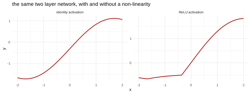
Figure 9.5: without activation, depth changes nothing
9.2.2 The sigmoid and the hyperbolic tangent
The two historical activations are the logistic function and the hyperbolic tangent:
\[\begin{align} \sigma(z)&=\frac{1}{1+e^{-z}} \in (0,1) \\ \tanh(z)&=\frac{e^{z}-e^{-z}}{e^{z}+e^{-z}} \in (-1,1) \tag{9.4} \end{align}\]
Both are smooth and bounded, which was considered a virtue: the activation of a neuron stays in a fixed range. The tanh is generally preferred to the sigmoid in the hidden layers because it is centred on zero, so its outputs do not all carry the same sign, which makes the following layer easier to train.
Their common defect is decisive, and it is read on their derivative. For the sigmoid, \(\sigma'(z)=\sigma(z)(1-\sigma(z))\), whose maximum is \(0.25\) at \(z=0\) and which collapses towards zero as soon as \(\lvert z\rvert\) exceeds a few units. A neuron that receives a large input is said to be saturated: its output barely moves, and above all the gradient that passes through it is almost null. In a deep network these small factors multiply, and the gradient vanishes before reaching the first layers.
9.2.3 ReLU and its variants
The rectified linear unit replaced them almost everywhere:
\[\begin{equation} ReLU(z)=\max(0,z) \tag{9.5} \end{equation}\]
Its derivative is \(1\) for \(z>0\) and \(0\) for \(z<0\). On the positive side it therefore transmits the gradient without attenuation, which is precisely what the sigmoid failed to do, and it costs a single comparison to compute. These two facts are the main reason why training deep networks became possible.
It has its own defect, the symmetric one: for \(z<0\) the gradient is exactly zero, and a neuron that has drifted into that region never comes back. This is called a dead neuron. The variants repair it by giving the negative side a small slope:
\[\begin{align} LeakyReLU(z)&=\max(\alpha z,z) \quad \text{with } \alpha \text{ small} \\ ELU(z)&=\begin{cases} z & z>0 \\ \alpha(e^{z}-1) & z\leqslant 0\end{cases} \\ GELU(z)&=z\,\Phi(z) \end{align}\]
where \(\Phi\) is the distribution function of the standard normal. The GELU, smoother, is the one used in most recent architectures.
In R:
z <- seq(-4, 4, length.out = 400)
acts <- list(
  sigmoid = list(f = function(z) 1 / (1 + exp(-z)),
                 d = function(z) { s <- 1 / (1 + exp(-z)); s * (1 - s) }),
  tanh    = list(f = function(z) tanh(z), d = function(z) 1 - tanh(z)^2),
  ReLU    = list(f = function(z) pmax(0, z), d = function(z) as.numeric(z > 0)),
  LeakyReLU = list(f = function(z) pmax(.1 * z, z),
                   d = function(z) ifelse(z > 0, 1, .1)),
  GELU    = list(f = function(z) z * pnorm(z),
                 d = function(z) pnorm(z) + z * dnorm(z)))

df_act <- do.call(rbind, lapply(names(acts), function(nm)
  rbind(data.frame(z, v = acts[[nm]]$f(z), act = nm, part = "activation g(z)"),
        data.frame(z, v = acts[[nm]]$d(z), act = nm, part = "derivative g'(z)"))))

ggplot(df_act, aes(z, v, colour = act)) +
  geom_line(linewidth = .9) +
  facet_wrap(~ part, ncol = 1, scales = "free_y") +
  geom_hline(yintercept = 0, colour = "grey70", linewidth = .3) +
  labs(title = "five activation functions", y = "") +
  theme_minimal()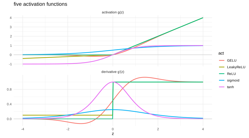
Figure 9.6: the activations and, above all, their derivatives
The lower panel is the important one, and it should be read with the training in mind. The derivative of the sigmoid never exceeds \(0.25\) and is close to zero outside a narrow band: multiply ten such factors and nothing is left. The derivative of the tanh reaches \(1\) but collapses just as fast. The derivative of the ReLU is exactly \(1\) over the whole positive half line, which is what lets the gradient travel through many layers, and exactly \(0\) on the other side, which is the price. The leaky variant and the GELU keep a non-zero derivative everywhere.
9.2.4 The output layer and the softmax
The hidden layers are free to use any activation, but the last one is imposed by the nature of the problem, exactly as the link function was in the generalized linear models of the chapter on non linear models:
regression: identity activation, the output is a real number, associated with a quadratic loss;
binary classification: sigmoid, the output is a probability, associated with the log loss;
multi-class classification: softmax, which turns \(K\) real scores into a probability distribution:
\[\begin{equation} softmax(z)_k=\frac{e^{z_k}}{\sum_{l=1}^{K}e^{z_l}} \tag{9.6} \end{equation}\]
The exponential makes everything positive and the denominator makes the sum equal to one. An important property is that the softmax depends only on the differences between the scores, since adding a constant to all of them changes nothing; this is used to subtract the maximum before exponentiating and avoid numerical overflow.
In Python:
import numpy as np
import pandas as pd
import matplotlib.pyplot as plt

def softmax(z):
    z = np.asarray(z, dtype=float)
    e = np.exp(z - z.max())          # the shift avoids the overflow
    return e / e.sum()

scores = np.array([2.0, 1.0, 0.1, -1.0])
probs = softmax(scores)

# the same scores divided by a temperature
temps = [0.5, 1.0, 3.0]
fig, axes = plt.subplots(1, 4, figsize=(11, 2.8))
axes[0].bar(range(4), scores, color="grey")
#> <BarContainer object of 4 artists>#> Text(0.5, 1.0, 'raw scores')for ax, T in zip(axes[1:], temps):
ax.bar(range(4), softmax(scores / T), color="steelblue")
ax.set_ylim(0, 1)
ax.set_title(f"softmax, T = {T}", fontsize=9)#> <BarContainer object of 4 artists>
#> (0.0, 1.0)
#> Text(0.5, 1.0, 'softmax, T = 0.5')
#> <BarContainer object of 4 artists>
#> (0.0, 1.0)
#> Text(0.5, 1.0, 'softmax, T = 1.0')
#> <BarContainer object of 4 artists>
#> (0.0, 1.0)
#> Text(0.5, 1.0, 'softmax, T = 3.0')plt.tight_layout(); plt.savefig("dl_softmax_py.png"); plt.clf(); plt.close()
softmax_tab = pd.DataFrame({"score": scores, "probability": np.round(probs, 4)})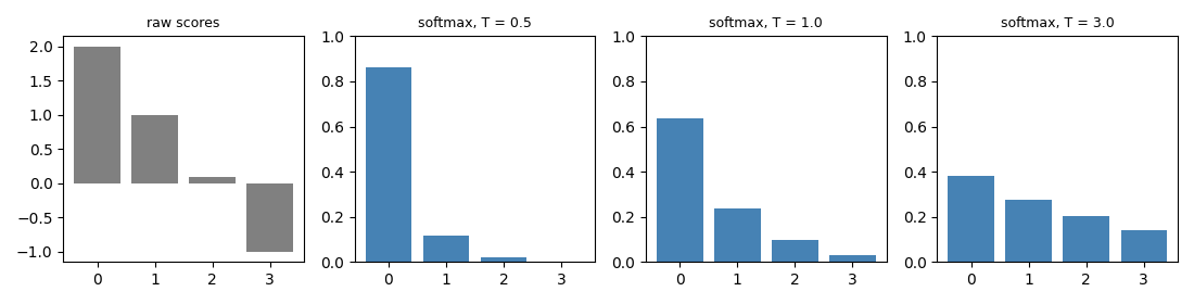
Figure 9.7: the softmax and the effect of the temperature
| score | probability |
|---|---|
| 2.0 | 0.6381 |
| 1.0 | 0.2347 |
| 0.1 | 0.0954 |
| -1.0 | 0.0318 |
The three right hand panels show the effect of dividing the scores by a temperature before applying the softmax. A low temperature sharpens the distribution until it almost designates a single class, a high temperature flattens it towards the uniform. This parameter plays no role during training, but it governs the diversity of the outputs when a trained network is used to generate text or images.