2.1 General concepts
The representation of relationships between economic processes as formal equations is the primary goal of the econometric field, provided that these equations will be the best possible interpretation of these real relationships, this set of equations combined called Model. By taking the case of supply and demand for a particular product assuming they only depend on the price of this product, so they can both of which written as a function of the price, it becomes easier to interpret the equilibrium of supply and demand by equations where their expressions are equal.
\[\begin{equation*} \begin{cases} S=f\left(p\right)\\ D=g\left(p\right)\\ S=D \end{cases} \end{equation*}\]
Supply and demand are not just related to the price. They may be affected by other variables like income or price of substitute goods, etc. Also, each variable may vary over time. Then these variables can be included in the above functions as follows:
\[\begin{equation*} \begin{cases} S_t=f\left(p_t, X_t, Y_t, ..\right)\\ D_t=g\left(p_t,X_t,Y_t,..\right)\\ S_t=D_t \end{cases} \end{equation*}\]
2.1.1 Random model
Suppose we want to study the consumption of a particular product by an individual t and assume that the consumption is affected only by the income of this individual. This relation then can be expressed by the following model:
\[\begin{equation*} C_t=f\left(R_t\right) \end{equation*}\]
Undoubtedly, other variables may be unknown (or maybe known but with small influence) may affect the consumption too. But if all these variables together have just a marginal effect, then they can be replaced by one random variable included in the model. This model, therefore, will be called a random model. The above model then will become:
\[\begin{equation*} C_t=f\left(R_t\right)+\varepsilon_t \end{equation*}\]
Where \(\varepsilon\) is called the disturbances term or error term.
The simplest form for this function is the simple linear function and recommended if the real relationship between two variables is nearly linear:
\[\begin{equation} C_t=\beta_0+\beta_1R_t+\varepsilon_t \tag{2.1} \end{equation}\]
Notice that, In this model, \(\beta_0\) and \(\beta_1\) are unknown constant parameters. The first one is called the intercept, and the second is called the slope. They cannot be computed exactly in any way from the data even though the data are all available, due to the random error in the model (unless for perfect deterministic relationship). Instead, they can be estimated using appropriate methods based on the statistical properties of random samples. If the sample is selected randomly from the population with enough observations, then it can be reliably used to estimate these parameters.
Definition 2.1 samples can be selected with three different forms:
- Time series : observations are collected over a period of time.
- Sectional data : observations are collected from different individuals , like persons or firms..etc, but with the same unit of time.
- Panel data : observations are collected from different individuals , like persons or firms..etc, and over time
Since the term estimation, by definition, is used when it is hard or impossible to get the exact values for the parameters, there exists a variety of estimation methods where each of which has its specific estimation criterion. For instance, one based on the differences between observations and estimated outcomes, another one is based on the shape of the population probability distribution, etc. Further, in this book, we will discuss the most popular of these methods.
Definition 2.2 The probability density and the distribution functions are defined by the following:
- \(f(X)\geqslant0\).
- \(\int\limits^{+\infty}_{-\infty}f(X)=1\).
- \(F(X)=P(X\leqslant x)=\int\limits^{x}_{-\infty}f(X)dX\).
- \(P(a\leqslant X \leqslant b)=\int\limits^{b}_{a}f(X)dX=F(b)-F(a)\).
2.1.2 Model variables
The basic econometric model has two types of variables:
Endogenous variable:
Other synonyms are Dependent variable, Regressand, Response. It is the variable of interest that we want to explain or to predict by using the explanatory variables included in the model. The main property of this variable is that when used in the model, it inherits some randomness from the random variable \(\varepsilon_t\) and hence becomes a random variable. In the model (2.1), the dependent variable is \(C_t\).
Exogenous variables:
Other synonyms are Explanatory variables, Independent variables, Regressors, Covariates, Predictors, etc. Conventionally, the use of each of which depends on the purpose of the model under study. If prediction, then we call these variables predictors. These variables are supposed to explain or predict the endogenous variable of the model and must be determined outside the model. in the model (2.1), \(R_t\) is an explanatory variable.
2.1.3 Estimation
Suppose, for simplicity, that the data generating process (DGP) characterizes a simple linear relationship between two variables but unknown to us, and we want to estimate this relationship by a linear equation (or the model) parameters. To obtain, thus, the best model, we should use the appropriate estimation method that provides the best possible accuracy. But since each one requires some data, we can collect this data by randomly sampling from the population (DGP) (if it is impossible to obtain all the population data). This idea comes from statistics based on the fact that the random samples are supposed to reflect the main aspects of the population.
If the model form correctly specified containing all the required explanatory variables, then said that the DGP is entirely known.
Unfortunately, even when the model is correctly specified, it is impossible to determine precisely the values of its parameters for two reasons: first, there may exist millions of factors that may affect this model. Second, in many cases, it is impossible to obtain all the DGP data. Therefore, all that we can do is to estimate this model using the collected samples from this DGP.
Assume that all we have from the underlying DGP is the sampled data set, which for simplicity, consists of only two variables, our variable of interest (The dependent variable) and the explanatory variable. The question is, how can we obtain the correct nature of the relationship between these two variables, or with other words, the right model specification. For our simple case, We can infer the theoretical relationship from the sample at hand using some statistical and visualization tools. However, This task would be very hard if we have a large number of variables due to the possible complex interactions among them.
The simple and the most effective way to investigate the nature of this relation in the sample is to plot the pair of observations that we have \((y_t,x_t),t=1,..,n\) to see whether the relationship is linear or has another shape. In the following R script, I have simulated some data to show q different types of relations.
Then I have used the most famous tool for visualizations ggplot(Wickham 2016), along with patchwork package used to organize several plots in the same panel in the form that we want. (The source code).
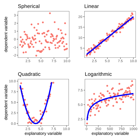
Figure 2.1: Type of Relations between two variables
We can see clearly that the upper right scatter plot is closer to the linear form, and hence it can be approximated by a straight line. While, the lower left one is closer to the quadratic shape, and the lower right one is closer to the logarithmic function. However, the latter plot seems to be also close to the linear form justifying the linear approximation. The last plot, obviously is too far from any shape indicating no relationship at all between these two variables.
Notice that any decision made, based only on the interpretation of these plots, is not always highly reliable since the scatter plot does not involve any statistic or probabilistic confidence levels. But plotting still be considered as the first insight into this relationship.
Visualize the data, if possible, maybe the first important step in estimation because it may recommend the best curve that fits the points. For instance, if these points are underlying closer to the logarithmic function curve, then this curve may be the best estimation of these data, and as the shape of the function now is known, it remains to look for its parameters.
In mathematics, the curve is derived from the function expression, but here the inverse is considered. That is the function expression that needs to be derived from the curve.
Starting with the investigation of the simple linear relation, if the shape of the points is closer to the linear function, then they can be approximated by a line. Here two important questions arise, the first is how the existing estimation methods work, and the second is how to choose the best of which.
2.1.4 Comparison of estimation methods
Let \(\theta\) be one of the DGP parameters, and let \(\widehat\theta\) be the estimator of this parameter, using one of the existing estimation methods, computed from the random sample as a function of the available observations \((y_t,x_t)\). Where \(y_t\) is a random variable (due to \(\varepsilon_t\)), which makes, in turn, \(\widehat\theta\) also as a random variable.
Given a specific sample, \(y_t\) is precisely known (from the observations), and the computed \(\widehat\theta\) is also known and called the estimate (or the outcome) of \(\theta\). However, randomness comes when the sample changes, that is, from sample to sample, the values of \(y_t\), and the estimates of \(\widehat\theta\) change randomly.
Now, intuitively, the more \(\widehat\theta\) is closer to \(\theta\), the more the estimation is accurate. In other words, the distance between the parameter and its estimator should tend to zero. In such case we say that the estimator is unbiased and can be interpreted in probability as \(p(\widehat\theta=\theta)\to1\). However, if we obtain two or more different estimators that are all unbiased, then we would choose the one that has less randomness (less variability) called then efficient estimator.
- Unbiased estimator:
The randomness of the estimator implies the existence of a particular distribution that depends on the DGP. Therefore, the distance can be defined by the difference between the mean of \(\widehat\theta\) and the unknown population parameter \(\theta\) with respect to the DGP distribution, that is \(E(\widehat\theta)-\theta\), so if \(E(\widehat\theta)-\theta=0\) then:
\[\begin{equation*} E(\widehat\theta)=\theta \end{equation*}\]
We say that the estimator is unbiased.
That is the first criterion used for comparison between estimation methods so that those that do not satisfy this property will be excluded, while the set of the remaining others with unbiased estimators will be called the class of unbiased estimators.
Efficient estimator:
If many estimators are all unbiased (centered around \(\theta\)), then, intuitively, that with the smallest volatility should be chosen, and this can be expressed by the so-called the mean squared error defined by :
\[\begin{equation*} MSE=E[(\widehat\theta-\theta)^2] \end{equation*}\]
Notice that this criterion must apply just with unbiased estimators:
\[\begin{equation*} MSE=E[(\hat\theta-\theta)^2]=V(\hat\theta)+[E(\hat\theta)-\theta]^2=V(\hat\theta) \end{equation*}\]
The efficient estimator is one that has a minimum variance within the class of unbiased estimators.
For the moment, we only investigate these criteria as we are with the simple linear regression. Further, we will introduce other ones with more complicated models.
Definition 2.3 (The Cramer-Rao lower bound) The lower bound variance of every unbiased estimator is given by:
- \(V(\widehat\theta)\geqslant\left(E\left[\left(\frac{(dlog(L(\theta))}{d\theta}\right)^2\right]\right)^{-1}=-\left(E\left[\left(\frac{(d^2log(L(\theta))}{d\theta^2}\right)\right]\right)^{-1}\)
Where \(L(\theta)\) is the likelihood func that will be introduced further.
That means the best efficient estimator is equal to this bound.