6.1 Non liner least squares regression NLS
When the model is non linear, the classical model \(y=X\beta\) under linear assumption, in a nonlinear form will be rewritten:
\[\begin{equation} y=\mathrm g(X, \beta)+\varepsilon \tag{6.1} \end{equation}\]
Using the least squares criterion, the objective function will be:
\[\begin{equation} S(\beta)=\sum\limits^n_{i=1}\big[y_i-\mathrm g(x_i, \beta)\big]^2+\varepsilon \tag{6.2} \end{equation}\]
Where \(x_i\) is the the \(i^{th}\) row of the matrix \(X\).
The minimization of this function should give us the best estimators we need. Assuming that the function \(\mathrm g\) is a continuous and differentiable equation, the first-order derivatives should equal to zero:
\[\begin{align} \frac{\partial S(\beta)}{\beta}&=-2\sum\limits^n_{i=1}\big[y_i-\mathrm g(x_i,\beta_{NLS})\big]\frac{\partial\mathrm g(x_i, \beta)}{\beta}\\ &=0 \tag{6.3} \end{align}\]
Those functions can be seen as the counterparts of the normal equations of the linear form.
The last expression \(\frac{\partial\mathrm g(x_i, \beta)}{\beta}\), that is equal to \(x_i\) in the linear regression, will be equal to what is called the pseudoregressors \(x_i^0\) in a nonlinear form(Green 2018). Thus, the above function will be rewritten:
\[\begin{align} \frac{\partial S(\beta)}{\beta}&=\sum\limits^n_{i=1}x_i^0\varepsilon\\ &=0 \tag{6.4} \end{align}\]
Some authors (such as Green) highlight the difference between the linear and nonlinear models in the functional form of Pseudo normal equation and not in the shape of the original model. If they are linear in \(\beta\), the original model is linear, even though nonlinear in the \(\beta\).
For solving the pseudo normal equations, we require iterative methods. The most used one is called Gauss-newton.
6.1.1 Gauss-Newton method
All the methods used to solve nonlinear functions are based on Taylor series approximation that decomposes the original function into small linear pieces.
This method uses an iterative process as follows:
- define an initial value \(\beta^0\).
- compute a new estimates \(\beta^1\).
- stop when no significant improvement in the objective function
The nonlinear function \(\mathrm g\), using this method will be approximated by:
\[\begin{align} \mathrm g(X, \beta) & \approx \mathrm g(X, \beta^0)+\sum\limits_{k=1}^K\frac{\partial\mathrm g(X, \beta^0)}{\partial\beta^0_k}(\beta_k-\beta^0_k) \\ & \approx\Bigg[\mathrm g(X, \beta^0)-\sum\limits_{k=1}^K\beta_k^0\frac{\partial\mathrm g(X, \beta^0)}{\partial\beta^0_k}\Bigg]+\sum\limits_{k=1}^K\beta_k\frac{\partial\mathrm g(X, \beta^0)}{\partial\beta^0_k} \tag{6.5} \end{align}\]
If we use only the firs order approximation (\(K=1\)), that function will be:
\[\begin{equation} \mathrm g(X, \beta) \approx\mathrm g(X, \beta^0)-\beta^0\frac{\partial\mathrm g(X, \beta^0)}{\partial\beta^0}+\beta\frac{\partial\mathrm g(X, \beta^0)}{\partial\beta^0} \tag{6.6} \end{equation}\]
Using again the pseudo regressors notations \(X^0\), the above function can be simplified to the following:
\[\begin{equation} \mathrm g(X, \beta) \approx \mathrm g(X, \beta^0)- X^0\beta^0+ X^0\beta \tag{6.7} \end{equation}\]
Substituting that equation into (6.1) and adding another error term \(\nu\) (assuming that it has the same assumptions as with \(\varepsilon\)) to the approximation, we get exact equality:
\[\begin{equation} y=\mathrm g(X, \beta^0)-X^0\beta^0+ X^0\beta+\overbrace{\varepsilon+\nu^0}^{\mu^0} \tag{6.8} \end{equation}\]
Since the first and the second members of the right hand side can be computed from the data at hand and the initialized value of \(\beta^0\), the above equation will be:
\[\begin{equation} \overbrace{y-\mathrm g(X, \beta^0)+ X^0\beta^0}^{y^0}= X^0\beta+\mu^0 \tag{6.9} \end{equation}\]
This model is linear now in \(\beta\), we can regress \(y^0\) on the pseudoregressors \(X^0\) using the classical linear least squares to obtain the first estimate \(\beta^1\) of the parameter vector \(\beta\):
\[\begin{equation} \beta^1_{NLS}=\big(X^{0t}X^0\big)^{-1}\big(X^{0t}y^0\big) \tag{6.10} \end{equation}\]
Then, in the next iteration, we will treat that estimate as \(\beta^0\) to generate another estimate, and so on until the estimates converge.
In general, at the \((h+1)^{th}\) iteration, the NLS estimators will be:
\[\begin{equation} \beta^{h+1}_{NLS}=\big(X^{ht}X^h\big)^{-1}X^{ht}y^h \tag{6.11} \end{equation}\]
And the residual vector of the nonlinear model (6.1) will be:
\[\begin{equation} e^h=y-\mathrm g\big(X, \beta^h_{NLS}\big) \tag{6.12} \end{equation}\]
Similar to \(y^0\) in (6.9), the \(y^h\) will be:
\[\begin{align} y^h&=y-\mathrm g(X, \beta^h_{NLS})+ X^h\beta^h_{NLS} \\ &= e^h+X^h\beta^h_{NLS} \tag{6.13} \end{align}\]
Finally, the estimate \(\beta^{h+1}_{NLS}\) resulted from regressing \(y^h\) on \(X^h\) will be computed as follows:
\[\begin{align} \beta^{h+1}_{NLS}&=\big(X^{ht}X^h\big)^{-1}X^{ht}y^h \\ &= \big(X^{ht}X^h\big)^{-1}X^{ht}\big(e^h+X^h\beta^h_{NLS}\big) \\ &=\beta^h_{NLS}+\big(X^{ht}X^h\big)^{-1}X^{ht}e^h \tag{6.14} \end{align}\]
As we see, the estimates get updated by the last term of the right hand side \(\big(X^{ht}X^h\big)^{-1}X^{ht}e^h\) that is resulted from regressing the residual vector from the last iteration on the pseudoregressors from the last iteration.
Example 6.1 Suppose that we have the following nonlineare model with one regressor:
\[\begin{equation*} y_i=\big(\alpha+\beta x_i\big)^{\gamma}+\varepsilon \end{equation*}\]
That is \(g(x, \alpha, \beta, \gamma)=\big(\alpha+\beta x\big)^{\gamma}\).
In the first step, we should set initial values for the parameters \((\alpha^0, \beta^0, \gamma^0)\).
Next we compute the residual vector \(e^0_i=y_i-\big(\alpha^0+\beta^0 x_i\big)^{\gamma^0}\) (since every thing is known)
Then, we compute the pseudoregressors evaluated at \((\alpha^0, \beta^0, \gamma^0)\):
\[\begin{align*} x^{0\alpha}_i&=\frac{\partial \mathrm g\big(x_i, \alpha, \beta, \gamma\big)}{\partial \alpha}=\gamma^0\big(\alpha^0+\beta^0x_i\big)^{\gamma^0 -1} \\ x^{0\beta}_i&=\frac{\partial \mathrm g\big(x_i, \alpha, \beta, \gamma\big)}{\partial\beta}=\gamma^0\big(\alpha^0+\beta^0x_i\big)^{\gamma^0 -1}x_i \\ x^{0\gamma}_i&=\frac{\partial \mathrm g\big(x_i, \alpha, \beta, \gamma\big)}{\partial \gamma}=\big(\alpha^0+\beta^0x_i\big)^{\gamma^0}ln\big(\alpha^0+\beta^0x_i\big) \end{align*}\]
Now we can regress the residual vector \(e_0\) on the pseudoregressor vector \(X^0=\begin{pmatrix}x^{0\alpha},x^{0\beta},x^{0\gamma} \end{pmatrix}^t\), then add the resulted estimates to the initial original values to obtain the new estimates of the model as follows:
\[\begin{equation*} \begin{pmatrix}\alpha^1_{NLS} \\ \beta^1_{NLS} \\ \gamma^1_{NLS} \end{pmatrix}= \begin{pmatrix}\alpha^0_{NLS} \\ \beta^0_{NLS} \\ \gamma^0_{NLS}\end{pmatrix}+\big(X^{0t}X^0\big)^{-1}X^{0t}e^0 \end{equation*}\]
6.1.2 Consistency of the NLS estimators
Like the linear models, the nonlinear models require similar assumptions to get consistent estimators(Green 2018).
Definition 6.1 (Assumptions of nonlinear models)
- A1: The functional form is nonlinear.
- A2: The vector mean of errors is equal to zero \(E(\varepsilon)=0\).
- A3: The variance of errors is constant \(E(\varepsilon^t)=\sigma^2\). This assumption is called Homoskedasticity.
- A4: No correlation between errors \(E(\varepsilon_t\varepsilon_s)=0\).
- These two last assumptions (3,4) can be rewritten together in matrix form: \(\Omega_{\varepsilon}=E(\varepsilon\varepsilon^t)=\sigma^2I_n\).
- A5: similar to the orthogonality condition in the linear model, the error term \(\varepsilon\) should be uncorrelated (not with \(X\)) with the pseudoregressors \(E\big(X^{0t}\varepsilon\big)=0\) .
- A6: The model parameters are all constant.
- A7: The errors are independentely and identically distributed \(\varepsilon\sim IID(0, \sigma^2I)\).
In addition to the above ones, we should have also:
- A8: To be estimable, the model parameter vactor must be identified (see the section 4.2.3.1).
- A9: The data generating process DGP should have a fixed first and second moments (at least) so that their counterparts in the sample converge to them.
it can be shown that the NLS estimators, under orthogonality condition (A5), are consistent provided that the matrix \(X^{ht}X^h\) (constructed from the pseudoregressors) converges to a finite matrix \(Q^h\). similar to the expressions (4.6) and (4.7), we should have:
\[\begin{equation} plim\frac{1}{n}\bigg(X^{ht}X^h\bigg)=plim\frac{1}{n}\sum\limits_{i=1}^n \Bigg(\frac{\partial\mathrm g\big(x_i, \beta^h\big)}{\partial\beta^{h}}\Bigg)\Bigg(\frac{\partial\mathrm g\big(x_i, \beta^h\big)}{\partial\beta^{ht}}\Bigg)=Q^h \tag{6.15} \end{equation}\]
\[\begin{equation} plim\frac{1}{n}\sum\limits_{i=1}^nX_i^h\varepsilon_i=0 \tag{6.16} \end{equation}\]
Let us start by including the plim operators into the expression (6.14). Using the orthogonality condition, that expression will be:
\[\begin{align} plim\bigg(\beta^{h+1}_{NLS}\bigg)&=plim\bigg(\beta^h_{NLS}\bigg)+\overbrace{plim\bigg(\big(X^{ht}X^h\big)^{-1}\bigg)}^{\big(Q^h\big)^{-1}}\overbrace{plim\bigg(X^{ht}e^h\bigg)}^{=0} \\ &=plim\bigg(\beta^h_{NLS}\bigg) \tag{6.17} \end{align}\]
That means the the two successive estimates should converge to the same value. Now, we hope that this value is the true \(\beta\) value.
Substituting the expression (6.12) into (6.11), we will obtain:
\[\begin{align*} \beta^{h+1}_{NLS}&=\beta^h_{NLS}+\big(X^{ht}X^h\big)^{-1}X^{ht}\big(y-\mathrm g\big(X, \beta^h_{NLS}\big) \\ &=\beta^h_{NLS}+\big(X^{ht}X^h\big)^{-1}X^{ht}y-\big(X^{ht}X^h\big)^{-1}X^{ht}\mathrm g\big(X, \beta^h_{NLS}\big) \\ &=\beta^h_{NLS}+\big(X^{ht}X^h\big)^{-1}X^{ht}\big(\mathrm g\big(X, \beta\big)+\varepsilon\big)-\big(X^{ht}X^h\big)^{-1}X^{ht}\mathrm g\big(X, \beta^h_{NLS}\big)\\ &=\beta^h_{NLS}+\big(X^{ht}X^h\big)^{-1}X^{ht}\mathrm g\big(X, \beta\big)+\big(X^{ht}X^h\big)^{-1}X^{ht}\varepsilon-\big(X^{ht}X^h\big)^{-1}X^{ht}\mathrm g\big(X, \beta^h_{NLS}\big) \\ \end{align*}\]
Including the plim operator, we will obtain:
\[\begin{align*} plim\bigg(\beta^{h+1}_{NLS}\bigg)&=plim\bigg(\beta^h_{NLS}\bigg)+\overbrace{plim\bigg(\big(X^{ht}X^h\big)^{-1}\bigg)}^{=\big(Q^h\big)^{-1}}X^{ht}\mathrm g\big(X, \beta\big) \\ &+\overbrace{plim\bigg(\big(X^{ht}X^h\big)^{-1}\bigg)}^{=\big(Q^h\big)^{-1}}\overbrace{plim\bigg(X^{ht}\varepsilon\bigg)}^{=0}-\overbrace{plim\bigg(\big(X^{ht}X^h\big)^{-1}\bigg)}^{=\big(Q^h\big)^{-1}}plim\bigg(X^{ht}\mathrm g\big(X, \beta^h_{NLS}\big)\bigg) \end{align*}\]
Using the result (6.17) and the orthogonality condition, the last expression will be:
\[\begin{equation*} \big(Q^h\big)^{-1}plim\bigg(X^{ht}\mathrm g\big(X, \beta^h_{NLS}\big)\bigg)=\big(Q^h\big)^{-1}X^{ht}\mathrm g\big(X, \beta\big) \end{equation*}\]
Finally, since the function \(\mathrm g\) is assumed to be continuous and identified, using the Continuous mapping theorem, the \(\beta^h_{NLS}\) converges to the true \(\beta\).
Definition 6.2 (Continuous mapping theorem) \(plim\big(\theta_n\big)=\theta\) if and only if \(plim\bigg(\mathrm g\big(\theta_n\big)\bigg)=\mathrm g\big(\theta\big)\)
where \(\theta_n\) and \(\theta\) are random variables, and \(\mathrm g\) is a continuous function.
If the errors are normally distributed, and using the same reasoning as in the linear model that yields the expression (4.10), we expect the distribution of the NLS estimators to follow also the normal distribution:
\[\begin{equation} \beta^h_{NLS}\overset{d}{\to}\mathrm N\bigg(\beta, \frac{1}{n}\sigma^2(Q^h)^{-1}\bigg) \tag{6.18} \end{equation}\]
Therefore, the asymptotic variance matrix will be:
\[\begin{equation} V_{Asy}\big(\beta_{NLS}^h\big)=\sigma^2_{NLS}\big(X^{ht}X^h\big)^{-1} \tag{6.19} \end{equation}\]
Where:
\[\begin{equation} \sigma^2_{NLS}=\frac{1}{n}\sum\limits_{i=1}^n\big[y_i-\mathrm g\big(x_i, \beta_{NLS}^h\big)\big]^2 \tag{6.20} \end{equation}\]
6.1.3 Hypothesis testing
As discussed in the section 3.9.2 from the chapter 2, we can group the most encountered restrictions as follows:
\[\begin{equation} H0:r(\beta)=q \tag{6.21} \end{equation}\]
Where the column vector \(r(\beta)\) has \(J\) functions representing the linear or nonlinear restrictions.
6.1.3.1 F-test in nonlinear models
To test those hypotheses, we can use the classical F-test that requires the estimation of the parameter vector of both models, the restricted one denoted \(\beta_{NLS}^*\) and the unrestricted one \(\beta_{NLS}\). Thus, the test will be:
\[\begin{equation} F(J, k)=\frac{\big(e^{*t}e^*-e^te\big)\big/J}{e^te\big/(n-k)} \tag{6.22} \end{equation}\]
It should be noted that both parts of the fraction follows the \(\chi^2\) distribution only by approximation.
6.1.3.2 Wald test in nonlinear models
As an alternative to F-test, the W-test uses the same expression (3.71). This test uses only the unrestricted model as follows:
\[\begin{equation} W=\big(r(\beta_{NLS})-q\big)^t\bigg[R(\beta_{NLS})V_{Asy}(\beta_{NLS})R^t(\beta_{NLS})\bigg]\big(r(\beta_{NLS})-q\big) \tag{6.23} \end{equation}\]
Where \(R(\beta)=\frac{\partial r(\beta)}{\partial \beta^t}\) is called the jacobien.
This test follows approximately the \(\chi^2\) distribution with \(J\) degrees of freedom.
6.1.3.3 Lagrange multiplier test in nonlinear models
Unlike the W-test, This test uses only the restricted model. Thus, if we note the pseudo regressors in the restricted model by \(X^h_*\), and the corresponding residuals by \(e_{*}\), then the LM-test will be:
\[\begin{equation} LM=\frac{e_*^tX_*^h\big(X^{ht}_*X^h_*\big)^{-1}X^{ht}_*Xe_*}{e_*^te_*\big/n} \tag{6.24} \end{equation}\]
Similar to W-test, this test also follows approximately the \(\chi^2\) distribution
In R:
We will use the function from the above example to generate some data.
# the population data
set.seed(11)
e <- rnorm(1000, 0, 0.5)
x <- seq(1, 50, length.out=1000)
y <- (1.5+15.6*x)^0.45+e
dfr_nls_pop <- tibble('y'=y, 'x'=x)

# take randomly 100 samples
set.seed(55)
dfr_nls <- dfr_nls_pop[sample(1:nrow(dfr_nls_pop), 100),]
head(dfr_nls)| y | x |
|---|---|
| 7.657579 | 3.991992 |
| 19.359460 | 49.313313 |
| 11.510534 | 12.918919 |
| 18.000830 | 34.059059 |
| 19.097221 | 43.966967 |
| 17.961489 | 38.669670 |
The following plot shows that the relationship is not linear.
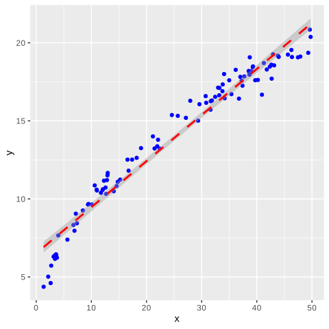
The true values are: \(\alpha=1.5\), \(\beta=15.6\), \(\gamma=0.45\). Now we will initiate the NLS estimations by: \(\alpha=0\), \(\beta=10\), \(\gamma=1\). The simple way to perform nonlinear least squares is by calling the base function nls as follows:
model_r_nls<-nls(y~(alpha+beta*x)^gamma,
                 start=list(alpha=0, beta=10, gamma=1),data=dfr_nls)
broom::tidy(model_r_nls)
[out] # A tibble: 3 × 5
[out] term estimate std.error statistic p.value
[out] <chr> <dbl> <dbl> <dbl> <dbl>
[out] 1 alpha 4.28 5.20 0.823 4.13e- 1
[out] 2 beta 15.8 3.20 4.93 3.35e- 6
[out] 3 gamma 0.449 0.0137 32.7 3.83e-54As we see the nls function accurately estimates \(\beta\) and \(\gamma\), but poorly estimates \(\alpha\).
We first move the data to python
In python we will use curve_fit function from scipy package as follows:
from scipy.optimize import curve_fit
import numpy as np

# we define the function we want to optimize
def myfunc(x, alpha, beta, gamma):
  return (alpha+beta*x)**gamma

curve_fit(myfunc, dfr_nls_py.x, dfr_nls_py.y, np.array([0, 10, 1]))
[out] (array([ 4.27660758, 15.8066471 , 0.44899113]), array([[ 2.70055817e+01, -1.43695977e+01, 6.03789285e-02],
[out] [-1.43695977e+01, 1.02657151e+01, -4.39783051e-02],
[out] [ 6.03789285e-02, -4.39783051e-02, 1.88917594e-04]]))the first line of this array contains the estimates. As we see we have obtained the same estimates such as those from R.