2.6 Regression with transformed variables
Sometimes, the variables we have cause some critical issues to the classical assumptions required to fit an OLS model. For instance, if the variable in question has a skewed distribution or some outliers, it may violate the normality assumption. Another case is when the relationship between the dependent variable and the explanatory variables is not linear. Sometimes, the variable does not cause any issue, but for interpretation purposes, the transformation is needed.
We will cover all the above issues and others in later chapters. But, here we will focus only on the most common transformations used in the OLS regression, the centered variables, the variables transformed with the power function, the logarithmic function, and lastly, the variables transformed with inverse hyperbolic sine function.
2.6.1 Centered variables
They are also called demeaned variables because derived from subtracting their means. We denote the centered variables by small letters as follows:
\[\begin{equation*} y_t=Y_t-\overline Y \qquad x_t=X_t-\overline X \end{equation*}\]
What happens to the OLS estimators if we use these transformed variables in place of the original ones? let us use the estimated model from (2.8):
\[\begin{equation*} \begin{cases} Y_t=\widehat \beta_0+\widehat \beta_1X_t+e_t\\ \overline Y=\widehat \beta_0+\widehat \beta_1\overline X+\underbrace{\overline e}_{=0} \end{cases} \implies\left(Y_t-\overline Y\right)=\widehat \beta_1\left(X_t-\overline X\right)+e_t\implies y_t=\widehat \beta_1x_t+e_t \end{equation*}\]
We see that \(\widehat \beta_1\) does not change, hence the interpretation of the resulted coefficients still the same. The original formula (2.12) with the new centered variables will be:
\[\begin{equation} \widehat \beta_1=\frac{\sum \left(Y_t-\overline Y\right)\left(X_t-\overline X\right)}{\sum \left(X_t-\overline X\right)^2}=\frac{\sum y_tx_t}{\sum x_t^2} \tag{2.56} \end{equation}\]
Even though the intercept disappears from the model, it is still computed using (2.11).
2.6.2 Polynomial transformation:
Sometimes the relationship between the dependent variable and the explanatory variable is not linear such as that in the lower left plot in the figure 2.1. So this relation should be presented by the following equation:
\[\begin{equation*} Y_t=\beta_0+\beta_1X^2_t+\varepsilon_t \end{equation*}\]
Notice that the relation indeed is not linear in terms of the explanatory variable \(X\), but it still linear in terms of the parameters \(\beta_0\) and \(\beta_1\) so that the linearity assumption still satisfied, hence the legitimate use of the OLS method.
If we replace \(X_t^2\) by \(Z\), then the OLS estimators in (2.11) and (2.12), will be:
\[\begin{equation*} \widehat \beta_0=\overline Y-\widehat \beta_1\overline Z \end{equation*}\]
\[\begin{equation*} \widehat \beta_1=\frac{\sum {Y_tZ_t}-n\overline Z\overline Y}{\sum Z_t^2-n\overline Z^2}=\frac{\sum {(Y_t-\overline Y_t)(X_t-\overline Z)}}{\sum (Z_t-\overline Z)^2} \end{equation*}\]
Substituting back \(X^2\), the OLS estimators for that model are given by:
\[\begin{equation*} \widehat \beta_0=\overline Y-\widehat \beta_1\overline {X^2} \end{equation*}\]
\[\begin{equation*} \widehat \beta_1=\frac{\sum {Y_tX^2_t}-n\overline {X^2}\overline Y}{\sum \bigg(X_t^2\bigg)^2-n\bigg(\overline {X^2}\bigg)^2}=\frac{\sum {\bigg(Y_t-\overline Y_t\bigg)\bigg(X^2_t-\overline {X^2}\bigg)}}{\sum \bigg(X^2_t-\overline {X^2}\bigg)^2} \end{equation*}\]
Where \(\overline {X^2}\) (not \(\overline {X}^2\)) is the mean of the transformed variable.
As a result, the interpretation of the slop now is different from that when we use the original variable. The marginal effect of \(X\) in the original model is:
\[\begin{equation*} \frac{\partial Y}{\partial X}=\widehat\beta_1 \end{equation*}\]
which is constant (under the classical assumptions).
However, with the transformed variable \(X^2\), the marginal effect of \(X\) becomes:
\[\begin{equation*} \frac{\partial Y}{\partial X}=2\widehat\beta_1X \end{equation*}\]
Now the marginal effect is no longer constant and depends on the magnitude of the variable \(X\). That is, the larger the \(X\) values, the larger the marginal effect.
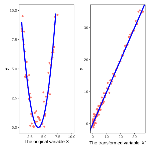
Figure 2.8: Regression with transformed variables
As shown in the above figure, the non linear relation transformed to linear one by squaring the original variable \(X\).
2.6.3 The Logarithmic transformation:
The logarithmic function is widely used to reduce the effect of the outliers, or to approximate the skewed distribution of the variable in question to the normal distribution.
Depending on the behavior of the variables we have, we have three possible cases, both variables (the dependent and the explanatory variables) needed to be log transformed, only the explanatory variable, and lastly only the dependent variable.
The linear-log model:
In this model only the explanatory variable \(X\) is transformed:
\[\begin{equation*} Y=\beta_0+\beta_1log(x)+\varepsilon \end{equation*}\]
The OLS estimators of this model then will be:
\[\begin{equation*} \widehat \beta_0=\overline Y-\widehat \beta_1\overline {log(X)} \end{equation*}\]
\[\begin{equation*} \widehat \beta_1=\frac{\sum {Y_tlog(X_t)}-n\overline {log(X)}\overline Y}{\sum log(X_t)^2-n\overline {log(X)}^2}=\frac{\sum {(Y_t-\overline Y_t)(X_t-\overline {log(X)})}}{\sum (log(X_t)-\overline {log(X)})^2} \end{equation*}\]
The marginal effect of the transformed variable \(log(X)\) (not the original one \(X\)) using this model is:
\[\begin{equation*} \frac{\partial Y}{\partial log(X)}=\widehat\beta_1 \end{equation*}\]
We can interpret \(\widehat\beta_1\) as the change in \(Y\) when \(log(X)\) increases by 1. But how can that coefficient relate to the original variable \(X\)? so using the following result:
\[\begin{equation} log(X)+1=log(X)+log(e)=log(Xe) \tag{2.57} \end{equation}\]
Where \(e\approx 2.73\) is the Euler number, we can deduce that adding 1 to the transformed variable \(log(X)\) is the same as multiplying the original variable \(X\) by \(2.73\). Therefore, we can say \(\widehat\beta_1\) is the change in \(Y\) when \(X\) is multiplied by \(2.73\).
We can derive the marginal effect of the original \(X\) directly from the model as follows:
\[\begin{equation*} \frac{\partial Y}{\partial X}=\frac{\widehat\beta_1}{X} \end{equation*}\]
As we see, the marginal effect varies with the values of \(X\), so that the higher the increase of \(X\), the smaller the increase in \(Y\). this behavior is the inverse of that of the polynomial function discussed above in which a high increase in \(X\) results in a high increase in \(Y\).
The log-linear model:
In this model we transform only the dependent variable \(Y\), while \(X\) still in its original form assuming that is well behaved:
\[\begin{equation*} log(Y)=\beta_0+\beta_1X+\varepsilon \end{equation*}\]
with this form, the estimators are given by:
\[\begin{equation*} \widehat \beta_0=\overline {log(Y)}-\widehat \beta_1\overline X \end{equation*}\]
\[\begin{equation*} \widehat \beta_1=\frac{\sum {log(Y_t)(X_t)}-n\overline X\overline {log(Y)}}{\sum X_t^2-n\overline X^2}=\frac{\sum {(log(Y_t)-\overline {log(Y)})(X_t-\overline X)}}{\sum (X_t-\overline X)^2} \end{equation*}\]
The marginal effect of the explanatory variable \(X\) on the dependent variable \(log(Y)\) (not the original one \(Y\)) will be written by:
\[\begin{equation*} \frac{\partial log(Y)}{\partial X}=\widehat\beta_1 \end{equation*}\]
we can interpret the coefficient \(\widehat\beta_1\) as the change in \(log(Y)\) (not \(Y\)) when \(X\) increases by 1. We can derive however the change in the original variable as follows:
\[\begin{equation} log\big(Y\big)+\widehat\beta_1=log\big(Y\big)+log\bigg(e^{\widehat\beta_1}\bigg)=log\bigg(Ye^{\widehat\beta_1}\bigg) \tag{2.58} \end{equation}\]
That means that when the explanatory variable \(X\) increases by one unit, then the resulted new value for the dependent variable is the the previous value multiplied by \(e^{\widehat\beta}\).
The estimated model can be written in terms of the original variable \(Y\) as follows:
\[\begin{equation*} log(Y)=\widehat\beta_0+\widehat\beta_1X+\widehat\varepsilon\implies Y=e^{(\widehat\beta_0+\widehat\beta_1X+\widehat\varepsilon)} \end{equation*}\]
Where \(\widehat\varepsilon\) stands for the residuals (to not confuse with Euler number \(e\)).
The marginal effect in terms of \(Y\) can be derived then as follows:
\[\begin{equation*} \begin{cases} \frac{\partial log( Y)}{\partial X}=\widehat\beta_1\\ \frac{\partial log( Y)}{\partial X}=\frac{\partial Y}{\partial X}.\frac{1}{Y} \end{cases} \implies\frac{\partial Y}{\partial X}=\widehat\beta_1Y=\widehat\beta_1e^{(\widehat\beta_0+\widehat\beta_1X+\widehat\varepsilon)} \end{equation*}\]
As we see, for fixed \(\widehat\beta_1\), a small increase in \(X\) results in higher increase in the change of \(Y\).
The log-log model:
In this model we transform both variables to the logarithmic form as follows:
\[\begin{equation*} log(Y)=\beta_0+\beta_1log(X)+\varepsilon \end{equation*}\]
with this form, the estimators are given by:
\[\begin{equation*} \widehat \beta_0=\overline {log(Y)}-\widehat \beta_1\overline {log(X)} \end{equation*}\]
\[\begin{equation*} \widehat \beta_1=\frac{\sum {log(Y_t)log(X_t)}-n\overline {log(X)}.\overline {log(Y)}}{\sum log(X_t)^2-n\overline {log(X)}^2}=\frac{\sum {(log(Y_t)-\overline {log(Y)})(log(X_t)-\overline {log(X)})}}{\sum (log(X_t)-\overline {log(X)})^2} \end{equation*}\]
We interpret \(\widehat\beta_1\) as the increase in \(log(y)\) when \(log(x)\) increases by 1 unit, and as we know from the linear-log model above (2.57), adding 1 to the transformed variable \(log(X)+1\) is equivalent to multiplying the original variable by \(e\approx2.73\), \(Xe\). Hence, by using the log-linear model (2.58), this will multiply the dependent variable by \(e^{\widehat\beta_1}\), \(Ye^{\widehat\beta_1}\).
In brief, if we multiply the explanatory variable \(X\) by \(e\), the variable \(Y\) will be multiplied by \(e^{\widehat\beta_1}\) in the log-log linear model.
However, there exists an equivalent straightforward simple interpretation. Since the marginal effect of this model in terms of the transformed variables \(log(Y)\) and \(log(X)\) is:
\[\begin{equation*} \frac{\partial log(Y)}{\partial log(X)}=\widehat\beta_1 \end{equation*}\]
It can be rewritten then in terms of the original variables \(Y\) and \(X\) as follows:
\[\begin{equation*} \frac{\partial log(Y)}{\partial log(X)}=\frac{\partial log(Y)\big/\partial X}{\partial log(X)\big/\partial X}=\frac{\frac{\partial Y}{\partial X}\frac{1}{Y}}{\frac{1}{X}}=\frac{\frac{\partial Y}{Y}}{\frac{\partial X}{X}}=\widehat\beta_1 \end{equation*}\]
As we see, \(\widehat\beta_1\) is the proportional change \(\frac{\partial Y}{Y}\) in the dependent variable when the proportional change \(\frac{\partial X}{X}\) in the explanatory variable increases by 1. In other words, if \(X\) increases by \(1\%\) then \(y\) will increase by \(\widehat\beta_1\%\). In economics, the coefficient of this model \(\widehat\beta_1\) is known as the elasticity of the variable \(Y\) with respect to the variable \(X\).
To derive the marginal effect of \(Y\) in terms of \(X\), let us first explicit \(Y\) in terms of \(X\) (without subscripts for simplification):
\[\begin{align*} &log(Y)=\widehat\beta_0+\widehat\beta_1log(X)+\widehat\varepsilon\\ &Y=e^{\widehat\beta_0+\widehat\beta_1log(X)+\widehat\varepsilon}\\ &Y=e^{(\widehat\beta_0+\widehat\varepsilon)}.X^{\widehat\beta_1} \end{align*}\]
Where the residual \(e\) is replaced by \(\widehat\varepsilon\) to distinguish it from the Euler number \(e\)
As said earlier, if we multiply \(X\) by \(e\), we expect the variable \(Y\) to be multiplied by \(e^{\widehat\beta_1}\). So let us verify it:
\[\begin{align*} Y_{new}&=e^{(\widehat\beta_0+\widehat\varepsilon)}.(Xe)^{\widehat\beta_1}\\ &=\overbrace{e^{(\widehat\beta_0+\widehat\varepsilon)}X^{\widehat\beta_1}}^{Y_{old}}e^{\widehat\beta_1}\\ Y_{new}&=Y_{old}e^{\widehat\beta_1} \end{align*}\]
By using the above results, the marginal effect of \(X\) on \(Y\) will be:
\[\begin{align*} &\frac{\partial log(Y)}{\partial log(X)}=\frac{\frac{\partial Y}{\partial X}\frac{1}{Y}}{\frac{1}{X}}=\frac{\partial Y}{\partial X}\frac{X}{Y}=\widehat\beta_1\\ &\frac{\partial Y}{\partial X}=\widehat\beta_1\frac{Y}{X}=\widehat\beta_1\frac{e^{(\widehat\beta_0+\widehat\varepsilon)}.X^{\widehat\beta_1}}{X}\\ &\frac{\partial Y}{\partial X}=\widehat\beta_1e^{(\widehat\beta_0+\widehat\varepsilon)}X^{(\widehat\beta_1-1)} \end{align*}\]
Although the logarithmic transformation is the most popular technique used in practice, it has few limitations. The major one is that it suffers from not being able to be used with the presence of zeroes or negative values. However, a common practice to solve this problem is by adding a constant with a small amount to the original variable in question to enable the use of this transformation. As shown in a paper2 written by(FENG et al. 2014), this solution can have a high effect on the significance of the null hypothesis.
2.6.4 The inverse hyperbolic sine transformation
This function, abbreviated as arcsinh, is an approximation of the logarithmic function with the advantage of retaining the zeroes and negative values. It is less known than the logarithmic function, but it gains popularity among practitioners over the logarithmic transformation.
The arcsinh function is given by:
\[\begin{equation*} X_{arcsinh}=ln(X+\sqrt{X^2+1}) \end{equation*}\]
As we see, this function is defined for all \(X\), because \(X+\sqrt{X^2+1}>0\) for all \(X\). We do not have thus to worry about the variable values as with the logarithmic transformation.
As we did with the logarithmic transformation, we will discuss three cases:
Definition 2.14 What we need to know about hyperbolic sine (sinh) and hyperbolic cosine functions (cosh) to understand this section is the following (restricted to \(\mathbb R\)):
- \(sinh(x)=\frac{e^x-e^{-x}}{2}\).
- \(cosh(x)=\frac{e^x+e^{-x}}{2}\).
- \(\frac{\partial sinh(x)}{\partial x}=cosh(x)\).
- \(\frac{\partial cosh(x)}{\partial x}=sinh(x)\).
- \(arcsinh=sinh^{-1}(x)=log(x+\sqrt{x^2+1})\).
- \(arccosh=cosh^{-1}(x)=log(x+\sqrt{x+1}\sqrt{x-1})\)
The linear-arcsinh model:
The linear model in terms of the transformed variable with the arcsinh function will be:
\[\begin{equation*} Y=\beta_0+\beta_1X_{arcsinh}+\varepsilon \end{equation*}\]
Then \(\widehat\beta_1\) is the change in \(Y\) when the transformed variable increases by 1:
\[\begin{equation*} log(X+\sqrt{X^2+1})+1=log(e(X+\sqrt{X^2+1})) \end{equation*}\]
That means that when the transformed variable \(log(X+\sqrt{X^2+1})\) increase by 1, then the new value of the explanatory variable can be derived from the following formula \(X_{new}+\sqrt{X_{new}^2+1}=e(X_{old}+\sqrt{X_{old}^2+1})\).
Since the estimated model is \(Y=\widehat\beta_0+\widehat\beta_1log(X+\sqrt{X^2+1})+\widehat\varepsilon\), then the marginal effect in terms of \(X\) is:
\[\begin{align*} \frac{\partial Y}{\partial X}&=\widehat\beta_1\frac{1+\frac{X}{\sqrt{X^2+1}}}{X+\sqrt{X^2+1}}\\ &=\frac{\big(X+\sqrt{X^2+1}\big)}{\sqrt{X^2+1}\big(X+\sqrt{X^2+1}\big)}\\ \frac{\partial Y}{\partial X}&=\frac{\widehat\beta_1}{\sqrt{X^2+1}} \end{align*}\]
For \(\widehat\beta_1\) fixed, each time \(X\) moves towards the positive infinite or the negative infinite, the change in \(Y\) becomes slower. In other words, the change in \(X\) when \(X\) has a high value (positive or negative) will not affect so much \(Y\). This result can be easily verified since \(\underset{X\to\mp\infty}{\lim}\frac{1}{\sqrt{X^2+1}}=0\).
The arcsinh-linear model:
This time, we only transform the dependent variable \(Y\) to be \(Y_{arcsinh}=log(Y+\sqrt{Y^2+1})\), the estimated model, in this case, will be:
\[\begin{equation*} Y_{arcsinh}=\widehat\beta_0+\widehat\beta_1X+\widehat\varepsilon \end{equation*}\]
In terms of \(Y_{arcsinh}\), When \(X\) increases by 1, the transformed variable \(Y_{arcsinh}\) increases by \(\widehat\beta_1\). However, in terms of the original variable \(Y\), By using the following equality:
\[\begin{equation*} log(Y+\sqrt{Y^2+1})+\widehat\beta_1=log\bigg(e^{\widehat\beta_1}\big(Y+\sqrt{Y^2+1}\big)\bigg) \end{equation*}\]
The new value of the dependent variable \(Y_{new}\) can be derived from the old value \(Y_{old}\) by the following formula:
\[\begin{equation*} Y_{new}+\sqrt{Y_{new}^2+1}=e^{\widehat\beta_1}\big(Y_{old}+\sqrt{Y_{old}^2+1}\big) \end{equation*}\]
First, let us reformulate the estimated model to which \(Y\) will be the dependent variable:
\[\begin{align*} \overbrace{arcsinh}^{sinh^{-1}}(Y)&=\widehat\beta_0+\widehat\beta_1X+\widehat\varepsilon\\ \overbrace{sinh(sinh^{-1}}^{\text{idendity function}}(Y))&=sinh(\widehat\beta_0+\widehat\beta_1X+\widehat\varepsilon)\\ Y&=sinh(\widehat\beta_0+\widehat\beta_1X+\widehat\varepsilon) \end{align*}\]
The marginal effect thus in terms of the original variables will be (see the definition #ref(def:sinh-cosh)):
\[\begin{equation*} \frac{\partial Y}{\partial X}=\widehat\beta_1cosh(\widehat\beta_0+\widehat\beta_1X+\widehat\varepsilon) \end{equation*}\]
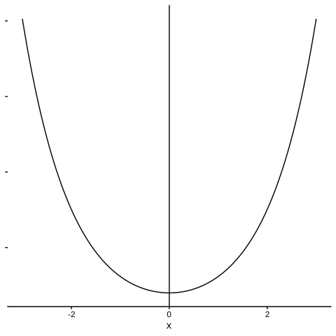
Figure 2.9: the cosinh function
The graph above shows that, for fixed \(\widehat\beta_1\), the marginal effect increases when \(X\) moves either, in the \(+\infty\) or the \(-\infty\) direction.
The arcsinh-arcsinh model:
The estimated model, whose variables are both transformed, with this form will be:
\[\begin{equation*} arcsinh(Y)=\widehat\beta_0+\widehat\beta_1arcsinh(X)+\widehat\varepsilon \end{equation*}\]
By applying the sinh function on both sides, the above model can be expressed in terms of \(Y\) as follows:
\[\begin{equation*} Y=sinh(\widehat\beta_0+\widehat\beta_1arcsinh(X)+\widehat\varepsilon) \end{equation*}\]
Hence, the marginal effect in terms of the original variables will be:
\[\begin{equation*} \frac{\partial Y}{\partial X}=\frac{\widehat\beta_1}{\sqrt{X^2+1}}.cosh(\widehat\beta_0+\widehat\beta_1arcsinh(X)+\widehat\varepsilon) \end{equation*}\]
As shown in a paper written by(Bellemare and Wichman 2020), \(\widehat\beta_1\) is an approximation of the elasticity derived from the log-log model with enough large values for \(X\) (more than 10).
This paper discusses some limitations of the logarithmic transformation with simulated data↩︎