9.7 Generative adversarial networks
The last architecture of the chapter answers a different question. Instead of predicting a label, it produces new observations resembling the training data, and it does so without anyone being able to write down what ‘resembling’ means. The solution, training two networks against each other, is one of the most elegant ideas of the field, and one of the most awkward to make work.
9.7.1 The adversarial idea
Everything so far was discriminative: given \(x\), predict \(y\). We now change the objective completely. We want to produce new observations that resemble those of the training set, without ever being told what “resemble” means.
The difficulty is exactly there. To train a model we need a loss, and here we cannot write one. What is the distance between a generated face and the set of all plausible faces? A pixel by pixel comparison is useless, since a face shifted by two pixels is still a face while being very far in that metric.
The idea of Goodfellow, in 2014, is to stop writing the loss and to learn it instead. Two networks are trained against each other:
the generator \(G\) takes a random vector \(z\) and produces a fake observation \(G(z)\);
the discriminator \(D\) receives an observation and outputs the probability that it is real.
The discriminator is trained to tell the two apart, and the generator is trained to fool the discriminator. Neither is ever told what a good sample looks like: the criterion is supplied by the opponent, and it becomes more demanding as the opponent improves.
9.7.2 Generator and discriminator
The generator maps a simple distribution, usually a standard normal in a space of a few dozen dimensions, onto the complicated distribution of the data. The vector \(z\) is called the latent code, and moving continuously in that space produces a continuous deformation of the output, which is one of the striking properties of these models.
The discriminator is an ordinary binary classifier. It has no special architecture; what is unusual is that its training set changes at every step, since the fakes it sees are produced by a generator that keeps improving.
In R:
boxes <- data.frame(
  x = c(0.6, 2.2, 2.2, 3.9),
  y = c(1.0, 1.55, 0.45, 1.0),
  lab = c("noise z", "generator G", "real data", "discriminator D"),
  fill = c("grey", "steelblue", "grey", "firebrick"))

arrows_df <- data.frame(
  x    = c(1.0, 2.62, 2.62, 4.3),
  y    = c(1.0, 1.55, 0.45, 1.0),
  xend = c(1.78, 3.5, 3.5, 4.75),
  yend = c(1.35, 1.12, 0.9, 1.0))

ggplot() +
  geom_segment(data = arrows_df, aes(x, y, xend = xend, yend = yend),
               arrow = arrow(length = unit(.16, "cm")), colour = "grey45") +
  geom_tile(data = boxes, aes(x, y, fill = fill), width = .85, height = .34,
            alpha = .25) +
  geom_text(data = boxes, aes(x, y, label = lab), size = 3.1) +
  geom_text(aes(4.95, 1.0, label = "real ?"), size = 3.1) +
  scale_fill_identity() +
  xlim(0, 5.4) + ylim(0.2, 1.8) +
  labs(title = "the generator never sees the real data directly",
       subtitle = "it only receives the gradient that passes through the discriminator") +
  theme_void() + theme(plot.subtitle = element_text(size = 9))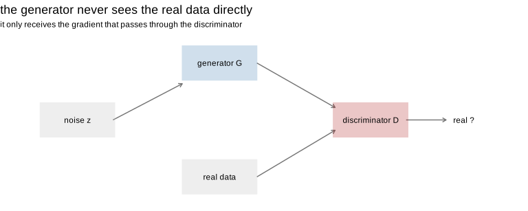
Figure 9.29: the two networks and the two flows of data
The subtitle states the point that is easiest to miss. The generator has no access to the real observations. Its only source of information is the gradient that flows back through the discriminator, which tells it in which direction to move its output so that the discriminator becomes a little more likely to be fooled.
9.7.3 The minimax objective
The two objectives are opposed, and they are written as a single two player game:
\[\begin{equation} \min_{G}\max_{D}\ \mathbb{E}_{x\sim p_{data}}\big[\ln D(x)\big]+\mathbb{E}_{z\sim p_{z}}\big[\ln\big(1-D(G(z))\big)\big] \tag{9.23} \end{equation}\]
The discriminator maximizes: it wants \(D(x)\) close to one on the real data and \(D(G(z))\) close to zero on the fakes. The generator minimizes the second term: it wants \(D(G(z))\) close to one.
Two remarks of practical importance. For a fixed generator, the optimal discriminator is \(D^*(x)=\frac{p_{data}(x)}{p_{data}(x)+p_g(x)}\), and substituting it shows that the generator is then minimizing the Jensen-Shannon divergence between the true distribution and its own. The game therefore does have a meaningful solution: \(p_g=p_{data}\).
But the second term of (9.23) saturates. At the beginning of training the generator is bad, \(D(G(z))\) is close to zero, and the gradient of \(\ln(1-D(G(z)))\) is almost flat, precisely when the generator most needs to learn. In practice one therefore maximizes \(\ln D(G(z))\) instead of minimizing \(\ln(1-D(G(z)))\), which has the same optimum and a much stronger gradient early on. This is the non-saturating loss, and it is what every implementation uses.
9.7.4 Why the training is difficult
A GAN does not minimize a function, it looks for an equilibrium between two moving objectives. The usual guarantees disappear, and the failure modes are specific.
Non-convergence and oscillation. The two networks may chase each other indefinitely, the generator moving towards what fooled the discriminator one step ago, which the discriminator has already corrected.
Mode collapse. The generator discovers a small region of output that fools the discriminator particularly well, and produces only that. It has minimized its loss while reproducing a fraction of the distribution. This is the most frequent failure and the easiest to see on a toy problem.
Imbalance. If the discriminator becomes too good, it rejects every fake with certainty, the gradient it returns vanishes, and the generator stops learning. If it is too weak, its signal is uninformative. The two must improve at comparable rates, which is why the learning rates and the number of updates of each are delicate.
The loss curves are unreadable in the usual way, and this must be said clearly: a decreasing generator loss does not mean the samples are improving, it may simply mean the discriminator has become weaker. GANs are evaluated by looking at the samples, and by quantitative scores designed for the purpose.
9.7.5 A worked example
We train a small GAN on a two dimensional distribution, a ring of eight gaussians. Working in two dimensions is what makes the mechanism and the failures visible, which images would not.
In Python:
#> <torch._C.Generator object at 0x0000020E2AABD510>rng_gan = np.random.default_rng(0)
# the target distribution: eight gaussians placed on a circle
def real_batch(n):
centres = np.stack([np.cos(np.linspace(0, 2*np.pi, 8, endpoint=False)),
np.sin(np.linspace(0, 2*np.pi, 8, endpoint=False))], 1) * 2.0
idx = rng_gan.integers(0, 8, n)
return (centres[idx] + rng_gan.normal(0, .12, (n, 2))).astype("float32")
LATENT = 8
G = nn.Sequential(nn.Linear(LATENT, 64), nn.ReLU(),
nn.Linear(64, 64), nn.ReLU(),
nn.Linear(64, 2))
D = nn.Sequential(nn.Linear(2, 64), nn.LeakyReLU(0.2),
nn.Linear(64, 64), nn.LeakyReLU(0.2),
nn.Linear(64, 1))
optG = torch.optim.Adam(G.parameters(), lr=2e-4, betas=(.5, .999))
optD = torch.optim.Adam(D.parameters(), lr=2e-4, betas=(.5, .999))
bce = nn.BCEWithLogitsLoss()
BS = 256
snapshots = {}
gan_hist = []
for step in range(1, 4001):
# --- discriminator
xr = torch.tensor(real_batch(BS))
z = torch.randn(BS, LATENT)
xf = G(z).detach()
optD.zero_grad()
lossD = bce(D(xr), torch.ones(BS, 1)) + bce(D(xf), torch.zeros(BS, 1))
lossD.backward(); optD.step()
# --- generator, non saturating loss
z = torch.randn(BS, LATENT)
optG.zero_grad()
lossG = bce(D(G(z)), torch.ones(BS, 1)) # maximize log D(G(z))
lossG.backward(); optG.step()
gan_hist.append({"step": step, "lossD": lossD.item(), "lossG": lossG.item()})
if step in (200, 800, 4000):
with torch.no_grad():
snapshots[step] = G(torch.randn(600, LATENT)).numpy()
gan_df = pd.DataFrame(gan_hist)real_show = real_batch(600)
fig, axes = plt.subplots(1, 4, figsize=(11, 2.9))
axes[0].scatter(real_show[:, 0], real_show[:, 1], s=4, color="black")#> <matplotlib.collections.PathCollection object at 0x0000020F2C9F1B50>#> Text(0.5, 1.0, 'real data')for ax, st in zip(axes[1:], [200, 800, 4000]):
g = snapshots[st]
ax.scatter(g[:, 0], g[:, 1], s=4, color="firebrick")
ax.set_title(f"generated, step {st}", fontsize=9)#> <matplotlib.collections.PathCollection object at 0x0000020F2CC3F590>
#> Text(0.5, 1.0, 'generated, step 200')
#> <matplotlib.collections.PathCollection object at 0x0000020F2CC3FBF0>
#> Text(0.5, 1.0, 'generated, step 800')
#> <matplotlib.collections.PathCollection object at 0x0000020F2C9C4170>
#> Text(0.5, 1.0, 'generated, step 4000')#> (-3.2, 3.2)
#> (-3.2, 3.2)
#> []
#> []
#> (-3.2, 3.2)
#> (-3.2, 3.2)
#> []
#> []
#> (-3.2, 3.2)
#> (-3.2, 3.2)
#> []
#> []
#> (-3.2, 3.2)
#> (-3.2, 3.2)
#> []
#> []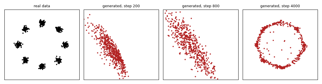
Figure 9.30: a GAN learning a ring of eight gaussians
The progression is readable. Early on the generator produces a shapeless cloud near the centre. It then finds the ring and begins to concentrate its output on it. At the end the eight modes are visible, more or less well covered.
The quantity worth measuring on this toy problem is precisely the coverage: how many of the eight modes the generator actually produces. It is computed by assigning each generated point to its nearest centre.
centres = np.stack([np.cos(np.linspace(0, 2*np.pi, 8, endpoint=False)),
                    np.sin(np.linspace(0, 2*np.pi, 8, endpoint=False))], 1) * 2.0

def coverage(pts, tol=.5):
    d = np.linalg.norm(pts[:, None, :] - centres[None, :, :], axis=2)
    nearest = d.argmin(1)
    close = d.min(1) < tol
    return len(np.unique(nearest[close])), float(close.mean())

cov_rows = []
for st, pts in snapshots.items():
    k, share = coverage(pts)
    cov_rows.append({"step": st, "modes_covered_out_of_8": k,
                     "share_of_points_near_a_mode": round(share, 3)})
gan_cov = pd.DataFrame(cov_rows)| step | modes_covered_out_of_8 | share_of_points_near_a_mode |
|---|---|---|
| 200 | 4 | 0.167 |
| 800 | 4 | 0.183 |
| 4000 | 8 | 0.778 |
#> <Figure size 700x300 with 0 Axes>#> [<matplotlib.lines.Line2D object at 0x0000020F2CC6E630>]#> [<matplotlib.lines.Line2D object at 0x0000020F2CC6F710>]#> Text(0.5, 0, 'step')
#> Text(0, 0.5, 'loss')
#> <matplotlib.legend.Legend object at 0x0000020F2C8FECC0>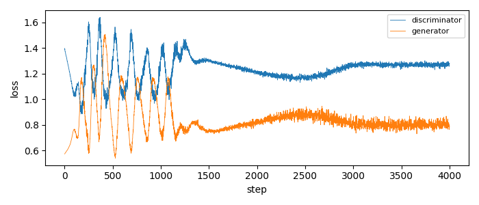
Figure 9.31: the adversarial losses
This last figure is the one to remember. The two curves oscillate around a level and neither of them descends towards zero, which would be alarming for any model of the previous chapters and is normal here: an equilibrium between two opponents is not a minimum. Judging a GAN by its loss curve is meaningless, and the only honest evaluation is the one we did just above, by looking at what it produces and measuring it.
The field has moved on considerably since. The Wasserstein GAN replaces the Jensen-Shannon divergence by a distance whose gradient does not vanish when the two distributions are disjoint, which greatly stabilizes the training; convolutional architectures and normalization of the weights of the discriminator did the rest. More recently, diffusion models, which learn to reverse a gradual addition of noise, have overtaken GANs on most image generation tasks, being far more stable to train. The adversarial principle presented here remains an essential idea, and it is used well beyond generation, for instance to make a representation independent of a sensitive variable.