3.2 Esimation by OLS method
Since each point in the multiple regression has \((k)\) coordinates \((y_t,x_{2t},x_{3t},..,x_{kt})\), it is impossible to visualize the scatter points in a space with a k dimension and hence verifying the linearity assumption. However, some posterior statistics exist to check this assumption, but we will not though discuss them right now.
In matrix form the OLS objective function becomes:
\[\begin{equation} S(\beta)=\sum \varepsilon_t^2=\varepsilon^t\varepsilon\quad where\quad t=transpose \tag{3.3} \end{equation}\]
Definition 3.1 Let \(A\) be the vector: \(A=\underset{(n\times1)}{\begin{pmatrix}a_1\\a_2\\..\\a_n\end{pmatrix}}\).
Its transpose is: \(A^t=\underset{(1\times n)}{(a_1,a_2,..,a_n)}\).
Its quadratic form is:
\[\begin{equation*}A^tA=\underset{(1\times n)}{(a_1,a_2,..,a_n)}\times \underset{(n\times1)}{\begin{pmatrix}a_1\\a_2\\..\\a_n\end{pmatrix}} =\underset{(1\times 1)}{\sum a_t^2}.\quad \text{It is a scalar} \end{equation*}\].
\(AA^t=\underset{(n\times1)}{\begin{pmatrix}a_1\\a_2\\..\\a_n\end{pmatrix}}\times \underset{(1\times n)}{(a_1,a_2,..,a_n)}=\underset{(n\times n)}{\begin{pmatrix}a_1^2&a_1a_2&..&a_1a_n\\a_2a_1&a_2^2&..&a_2a_n\\..&..&..&..\\a_na_1&a_na_2&..&a_n^2\end{pmatrix}}\quad \text{It is symmetric}\).
\((A+B)^t=A^t+B^t\quad, \quad (AB)^t=B^tA^t \quad, \quad (A^t)^t=A\).
To be defined, a product of two matrices requires that the column number of the first matrix is equal to the row number of the second matrix.
Substituting (3.2) in (3.3) we get:
\[\begin{align*} S(\beta)=\varepsilon^t\varepsilon&=(y-X\beta)^t(y-X\beta)\\ &=(y^t-\beta^tX^t)(y-X\beta)\\ &=y^ty-y^tX\beta-\beta^tX^ty+\beta^tX^tX\beta \end{align*}\]
Note that the result is a scalar since each member of the last expression has a scalar value. By using the transpose properties, we find that \((y^tX\beta)^t=\beta^tX^ty\) because both sides are scalars, and the transpose of a scalar equals to itself. Thus, the last expression will be:
\[\begin{equation*} S(\beta)=y^ty-2\beta^tX^ty+\beta^tX^tX\beta \end{equation*}\]
To get the minimum of this expression, we have to set the derivatives with respect to the vector \(\beta\) to zero, and as \(\beta\) has \(k\) components, we should get \(k\) equations summarized in matrix form as follows:
\[\begin{equation*} \frac{\partial S}{\partial \beta}=-2X^ty+2(X^tX)\widehat\beta=0 \end{equation*}\]
Henceforth, since we will discuss different kinds of estimators in the scope of this book, \(\widehat\beta\) will always refer to the OLS estimators unless indicated otherwise.
Typically, the last expression gives \(k\) normal equations
\[\begin{equation} (X^tX)\widehat\beta=X^ty \tag{3.4} \end{equation}\]
with more detail:
\[\begin{equation} \underset{(k\times k)}{\begin{pmatrix} n&\sum x_{2t}&\sum x_{3t}&..&\sum x_{kt}\\ \sum x_{2t}&\sum x_{2t}^2&\sum x_{2t}x_{3t}&..&\sum x_{2t}x_{kt}\\ \sum x_{3t}&\sum x_{3t}x_{2t}&\sum x_{3t}^2&..&\sum x_{3t}x_{kt}\\ ..&..&..&..&..\\ \sum x_{kt}&\sum x_{kt}x_{2t}&\sum x_{kt}x_{3t}&..&\sum x_{kt}^2 \end{pmatrix}} \underset {(k\times 1)} {\begin{pmatrix} \widehat\beta_1\\ \widehat\beta_2\\ \widehat\beta_3\\ ..\\ \widehat\beta_K \end{pmatrix}}= \underset {(k \times 1)} {\begin{pmatrix} \sum y_t\\ \sum x_{2t}y_t\\ \sum x_{3t}y_t\\ ..\\ \sum x_{kt}y_t \end{pmatrix}} \tag{3.5} \end{equation}\]
Definition 3.2 Properties of the matrix \(X^tX\):
- The matrix \(X^tX\) is symmetric.
- We read the sample size \(n\) from the top left corner of this matrix.
- After dividing the first row (or the first column) by \(n\), each element is the sample mean of the corresponding regressor.
- After dividing the first element of the vector \(X^ty\), we get the dependent variable sample mean.
Finally, the estimator vector is given by:
\[\begin{equation} \widehat\beta=(X^tX)^{-1}(X^ty) \tag{3.6} \end{equation}\]
Provided that the matrix \(X^tX\) is invertible. Otherwise, This expression has no solution meaning that OLS is unable to give an estimator in such a situation. knowing the requirements that make a matrix invertible will help to find ways for manipulating our matrix \(X^tX\).
We know from matrices algebra that an invertible matrix has its determinant different from zero, and hence it is a full rank matrix. The determinant will be equal to zero if any linear combination among rows or columns exists. Therefore, the matrix \(X^tX\) must have a full rank \(k\), but as \(X\) is \((n\times k)\) matrix, the number of observations must be greater than the number of parameters \(k\) or at least equal to it \(k\leqslant n\). Moreover, For its determinant to be different from zero, it must not exist any linear combination among rows or columns.
In practice, it is rare when detecting a perfect linear relation between regressors. But, statistically, regressors instead can have strong (not perfect) linear correlations between them. Therefore, the strong correlations between regressors push the determinant to zero, and then the invertible matrix \((X^tX)^{-1}\) to infinite. The presence of such correlations between regressors is called multicollinearity. That is why we will add the absence of multicollinearity as a new assumption to the rest of our assumptions.
3.2.1 The estimated model:
The estimated model in multiple linear regression can be written as:
\[\begin{equation} y=X\widehat\beta+e \tag{3.7} \end{equation}\]
Where \(e\) is the sample error vector called residual vector.
The vector of the fitted values is:
\[\begin{equation} \widehat y=X\widehat\beta \tag{3.8} \end{equation}\]
In some situations, we need to express the fitted values vector in terms only of the observations by substituting (3.6) in the last expression as follows:
\[\begin{align} \widehat y&=X\widehat\beta=X(X^tX)^{-1}X^ty\notag\\ \widehat y&=\underset{(n\times n)}{H}y \tag{3.9} \end{align}\]
Where \(H=X(X^tX)^{-1}X^t\) is called hat matrix.
The residual vector can also be expressed in terms of observations:
\[\begin{align} e&=y-X\widehat\beta=y-X(X^tX)^{-1}X^ty\notag\\ e&=(I_n-X(X^tX)^{-1}X^t)y\notag\\ e&=\underset{(n\times n)}{M}y \tag{3.10} \end{align}\]
Where \(M=(I-X(X^tX)^{-1}X^t)\) is \((n\times n)\) matrix, and \(I_n\) is the identity matrix with n dimensions.
Definition 3.3 (Properties of M and H) Properties of \(M\) and \(H\):
- Summing \(M\) with \(H\) gives the indentity matrix:
\[\begin{equation*} M=I-X(X^tX)^{-1}X^t=I-H\implies M+H=I \end{equation*}\]
- Multiplying \(M\) by \(H\) gives zero:
\[\begin{align*} MH&=(I-X(X^tX)^{-1}X^t)X(X^tX)^{-1}X^t\\ &=X(X^tX)^{-1}X^t-X(X^tX)^{-1}\underbrace{X^tX(X^tX)^{-1}}_{I_n}X^t\\&=X(X^tX)^{-1}X^t-X(X^tX)^{-1}X^t\\ &=0 \end{align*}\]
- The matrix \(M\) is symmetric:
\[\begin{equation*} M^t=(I_n-X(X^tX)^{-1}X^t)^t=I_n-X(X^tX)^{-1}X^t=M \end{equation*}\]
- The matrix \(M\) is idempotent:
\[\begin{align*} M^2=MM&=(I_n-X(X^tX)^{-1}X^t)(I_n-X(X^tX)^{-1}X^t)\\ &=I_n-X(X^tX)^{-1}X^t-X(X^tX)^{-1}X^t+X(X^tX)^{-1}\underbrace{X^tX(X^tX)^{-1}}_{=I_n}X^t\\&=I_n-X(X^tX)^{-1}X^t\\ &=M \end{align*}\]
- Multiplying \(M\) with \(X\) gives zero:
\[\begin{align*} MX&=(I_n-X(X^tX)^{-1}X^t)X\\ &=X-X(X^tX)^{-1}X^tX\\ &=X-X\\ &=0 \end{align*}\]
- Premultiplying \(e\) by \(M\) does not change \(e\):
\[\begin{align*} Me&=M(y-X\widehat\beta)\\ &=My-\underbrace{MX}_{=0}\widehat\beta\\ &=My\\ &=e \end{align*}\]
- The matrix \(H\) is symmetric:
\[\begin{equation*} H^t=\big(X(X^tX)^{-1}X^t\big)^t=X(X^tX)^{-1}X^t=H \end{equation*}\]
- The matrix \(H\) is idempotent:
\[\begin{align*} H^2&=HH=X(X^tX)^{-1}\underbrace{X^tX(X^tX)^{-1}}_{=I_n}X^t\\ &=X(X^tX)^{-1}X^t\\ &=H \end{align*}\]
If we explicit (3.4) further, we get the orthogonality condition between the residual vector and the regressors vector:
\[\begin{equation} (X^tX)\widehat\beta=X^ty=X^t(X\widehat\beta+e)=(X^tX)\widehat\beta+X^te\implies X^te=0 \tag{3.11} \end{equation}\]
Using this result, we can prove that the residual vector is also orthogonal to the fitted values vector \(\widehat Y\):
\[\begin{equation} \widehat y^te=(X\widehat \beta)^te=\widehat \beta^t\underbrace{X^te}_{=0}=0 \tag{3.12} \end{equation}\]
3.2.2 The means of the OLS estimators
From what we learned from the previous chapter, we have to check the unbiasedness and the efficiency of our estimators. Since combined into a single vector, we use matrix algebra to compute the corresponding vector of means and the variance matrix.
Each component of this vector is a single mean:
\[\begin{equation*} E(\widehat\beta)= \underset{(k\times 1)} {\begin{pmatrix} E(\widehat\beta_1)\\ E(\widehat\beta_2)\\ ..\\ E(\widehat\beta_k) \end{pmatrix}} \end{equation*}\]
Substituting (3.2) in (3.6), we get:
\[\begin{align} \widehat\beta=(X^tX)^{-1}X^ty&=(X^tX)^{-1}X^t(X\beta+\varepsilon)\notag\\ &=\underbrace{(X^tX)^{-1}(X^tX)}_{=I_n}\beta+(X^tX)^{-1}X^t\varepsilon\notag\\ &=\beta+(X^tX)^{-1}X^t\varepsilon \tag{3.13} \end{align}\]
By including then the expectation operator, the mean will be:
\[\begin{equation*} E(\widehat\beta)=\beta+(X^tX)^{-1}X^t\overbrace{E(\varepsilon)}^{=0} \end{equation*}\]
\[\begin{equation} E(\widehat\beta)=\beta \tag{3.14} \end{equation}\]
That means that the OLS estimator \(\widehat\beta\) is unbiased. Note that unbiasedness requires the two first assumptions, the non-random regressors assumption that allows the expectation operator to skip the expression \((X^tX)^{-1}X^t\), and the zero errors mean \(E(\varepsilon)=0\).
3.2.3 The variance matrix of the OLS estimators
The variance matrix of the estimators can be defined as:
\[\begin{align*} Var(\widehat\beta)&=E\bigg[(\widehat\beta-\beta)(\widehat\beta-\beta)^t\bigg]\\ &= \begin{pmatrix} V(\widehat\beta_1)&cov(\widehat\beta_1,\widehat\beta_2)&..&cov(\widehat\beta_1,\widehat\beta_k)\\ cov(\widehat\beta_2,\widehat\beta_1)&V(\widehat\beta_2)&..&cov(\widehat\beta_2,\widehat\beta_k)\\ ..&..&..&..\\ cov(\widehat\beta_k,\widehat\beta_1)&cov(\widehat\beta_k,\widehat\beta_2)&..&V(\widehat\beta_k) \end{pmatrix} \end{align*}\]
Note that the position of each single estimator variance in the above matrix diagonal match the corresponding estimator position in the estimated model (3.7).
Substituting (3.13) in the last variance formula, we get:
\[\begin{align} Var(\widehat\beta)&=E\bigg[(\widehat\beta-\beta)(\widehat\beta-\beta)^t\bigg]\notag\\ &=E\bigg[\bigg((X^tX)^{-1}X^t\varepsilon\bigg)\bigg((X^tX)^{-1}X^t\varepsilon\bigg)^t\bigg]\notag\\ &=E\bigg[(X^tX)^{-1}X^t\varepsilon\varepsilon^tX(X^tX)^{-1}\bigg]\notag\\ &=(X^tX)^{-1}X^tE(\varepsilon\varepsilon^t)X(X^tX)^{-1} \tag{3.15} \end{align}\]
The expression \(E(\varepsilon\varepsilon^t)\) in the middle is the variance matrix of errors that will be denoted \(\Omega_{\varepsilon}\). It has the following elements:
\[\begin{equation*} \underset{(n\times n)}{\Omega_{\varepsilon}}=E(\varepsilon\varepsilon^t)=E \begin{pmatrix} \overbrace{E(\varepsilon_1^2)}^{=\sigma^2}&\overbrace{E(\varepsilon_1\varepsilon_2)}^{=0}&..&E(\varepsilon_1\varepsilon_2)\\ E(\varepsilon_2\varepsilon_1)&E(\varepsilon_2^2)&..&E(\varepsilon_2\varepsilon_n)\\ ..&..&..&..\\ E(\varepsilon_n\varepsilon_1)&E(\varepsilon_n\varepsilon_2)&..&E(\varepsilon_n^2) \end{pmatrix} \end{equation*}\]
Using assumptions \(A3\) and \(A4\), see 2.8, this matrix can be reduced to:
\[\begin{equation} \Omega_{\varepsilon}=\sigma^2I_n \tag{3.16} \end{equation}\]
Substituting this result in (3.15), we get:
\[\begin{align*} Var(\widehat\beta)&=(X^tX)^{-1}X^t\Omega_{\varepsilon}X(X^tX)^{-1}\\ &=\sigma^2\underbrace{(X^tX)^{-1}X^tX}_{=I_n}(X^tX)^{-1} \end{align*}\]
Finally, the variance of \(\widehat\beta\) will be written:
\[\begin{equation} Var(\widehat\beta)=\sigma^2(X^tX)^{-1} \tag{3.17} \end{equation}\]
As said earlier, the best estimator should have the smallest variance. Thus, if the multicollinearity assumption is not satisfied, the matrix value \((X^tX)^{-1}\) would be substantially high, which leads to a higher variance and hence undermines the OLS estimators efficiency.
3.2.4 Estimation of the error variance
Intuitively, The variance of the residuals can be a good candidate estimator of the theoretical error variance. Using \(MX=0\) (see 3.3), the error vector \(e\) can be expressed in terms of \(\varepsilon\) as follows:
\[\begin{align*} e&=My=\overbrace{MX}^{=0}\beta+M\varepsilon\\ e&=M\varepsilon \end{align*}\]
The sum of squared errors can be written in matrix form as:
\[\begin{equation*} \sum e_t^2=e^te=(M\varepsilon)^tM\varepsilon=\varepsilon^t\overbrace{M^tM}^{=M}\varepsilon \end{equation*}\]
Using the properties of \(M\) (see 3.3), it follows that:
\[\begin{equation} e^te=\varepsilon^tM\varepsilon \tag{3.18} \end{equation}\]
In more depth, that expression can be rewritten in terms of the elements of \(M\), denoted \(m_{ij}\), as follows:
\[\begin{equation*} e^te=\varepsilon^tM\varepsilon=\sum\limits_im_{ii}\varepsilon_i^2+\sum\limits_i\sum\limits_jm_{ij}\varepsilon_i\varepsilon_j \end{equation*}\]
Including then the expectation operator and using assumptions \(A3\) and \(A4\). see 2.8:
\[\begin{align*} E(e^te)&=\sum\limits_im_{ii}\overbrace{E(\varepsilon_i^2)}^{=\sigma^2}+\sum\limits_i\sum\limits_jm_{ij}\overbrace{E(\varepsilon_i\varepsilon_j)}^{=0}\\ &=\sigma^2\sum\limits_im_{ii}\\ &=\sigma^2Tr(M)\quad,\quad Tr=\text{Trace} \end{align*}\]
Let us now check the trace of the matrix \(M\) by using the properties of the \(Tr\) operator:
\[\begin{align} Tr(M)&=Tr\bigg(I_n-X(X^tX)^{-1}X^t\bigg)\notag\\ &=Tr(I_n)-Tr\bigg(X(X^tX)^{-1}X^t\bigg)\notag\\ &=Tr(I_n)-Tr\bigg(\underbrace{X^tX(X^tX)^{-1}}_{=I_k}\bigg)\notag\\ &=Tr(I_n)-Tr(I_k)\notag\\ Tr(M)&=n-k \tag{3.19} \end{align}\]
Substituting this result into the above expression, we get:
\[\begin{equation*} E(e^te)=\sigma^2(n-k) \end{equation*}\]
It is easy to show that the variance of the residuals is not unbiased:
\[\begin{equation*} E(\sigma^2_e)=E\bigg(\frac{e^te}{n}\bigg)=\sigma^2\frac{n-k}{n} \end{equation*}\]
However, an unbiased estimator can be easily derived from this expression as follows:
\[\begin{equation*} E\bigg(\frac{e^te}{n-k}\bigg)=\sigma^2\implies \end{equation*}\]
\[\begin{equation} s^2=\frac{e^te}{n-k} \tag{3.20} \end{equation}\]
The square root of this variance \(s\) is called, The standard error of regression.
Notice that this unbiased variance \(s^2\) is larger than the classical sample error variance \(\sigma^2_e\) because of the denominator of the former \(n-k\) that is smaller than \(n\).
3.2.5 The variance analysis equation
Let us split the matrix \(X\) into two disjoint blocks, the first one holds a vector of ones referred to the constant terms denoted \(i\), and the second block the regressor denoted \(X_2\):
\[\begin{equation*} X=\big(iX_2\big) \end{equation*}\]
Its transpose hence is:
\[\begin{equation*} X^t= \begin{pmatrix} i^t\\ X^t_2 \end{pmatrix} \end{equation*}\]
Using this formulation now, we can prove that the sample residuals mean \(\overline e\) is zero.
\[\begin{equation} X^te= \begin{pmatrix} i^t\\ X^t_2 \end{pmatrix} e= \begin{pmatrix} i^te\\ X^t_2e \end{pmatrix} = \begin{pmatrix} 0\\ 0 \end{pmatrix} \tag{3.21} \end{equation}\]
The first component can be used to prove that \(\overline{\widehat y}=\overline y\) as follows:
\[\begin{equation*} \begin{cases} \overline{\widehat y}=\widehat\beta_1+\widehat\beta_2\overline x_2+\widehat\beta_3\overline x_3+..+\widehat\beta_K\overline x_k\\ \overline y=\widehat\beta_1+\widehat\beta_2\overline x_2+\widehat\beta_3\overline x_3+..+\widehat\beta_K\overline x_k+\underbrace{\overline e}_{=0} \end{cases} \implies\overline{\widehat y}=\overline y \end{equation*}\]
Using this property, the total sum of squares and the explained sum of squares can be rewritten in matrix form:
\[\begin{equation*} \begin{cases} SST=\sum \left(y_t-\overline y\right)^2=\sum y_t^2-n\overline y^2=y^ty-n\overline y^2\\ SSE=\sum \left(\widehat y_t-\overline y\right)^2=\sum \widehat y_t^2-n\overline y^2=\widehat y^t\widehat y-n\overline y^2 \end{cases} \end{equation*}\]
However, there exists another interesting formulation for the sums that is helpful in some circumstances as the following:
\[\begin{equation} \sum \left(y_t-\overline y\right)^2=y^tNy \tag{3.22} \end{equation}\]
Where
\[\begin{equation} N=I_n-i(i^ti)^{-1}i^t=I_n-\frac{1}{n}ii^t \tag{3.23} \end{equation}\]
This matrix can be seen as the matrix \(M\) where \(X=i\), from which it inherits all the properties of \(M\) such as:
\(Ni=\big(I_n-i(i^ti)^{-1}i^t\big)i=i-i\overbrace{(i^ti)^{-1}i^ti}^{=I_n}=0\).
\(Ne=\big(I_n-i(i^ti)^{-1}i^t\big)e=e-i(i^ti)^{-1}\overbrace{i^te}^{=0}=e\).
That means that the sum of squared residuals does not change:
- \(e^tNe=e^te\).
Let us now explicit \(y^ty\) in terms of \(\widehat y\) and \(e\) and using the orthogonality between them (see (3.12)):
\[\begin{align*} y^ty&=(\widehat y+e)^t(\widehat y+e)\\ &=\widehat y^t\widehat y+\overbrace{\widehat y^te}^{=0}+\overbrace{e^t\widehat y}^{=0}+e^te\\ &=\widehat y^t\widehat y+e^te \end{align*}\]
Subtracting \(n\overline y^2\) from each side, we get the variance analysis equation:
\[\begin{equation} \underbrace{y^ty-n\overline y^2}_{SST}=\underbrace{\widehat y^t\widehat y-n\overline y^2}_{SSE}+\underbrace{e^te}_{SSR} \tag{3.24} \end{equation}\]
From this formula, we can set up the variance analysis table:
| Source of variance | sum of squares | Degrees of freedom | The mean of squares |
|---|---|---|---|
| Y | \(SST=y^ty-n\overline y^2\) | \(n-1\) | \(\frac{SST}{n-1}\) |
| X | \(SSE=\widehat y^t\widehat y-n\overline y^2\) | k-1 | \(\frac{SSE}{k-1}\) |
| e | \(SSR=e^te\) | \(n-k\) | \(\frac{SSR}{n-k}\) |
Example 3.1 In this example, we will simulate a data set that contains only a numeric variables.
set.seed(1)

# generate 100 normal variables with mean zero
# and standard deviation 5
epsilon <- rnorm(100, 0, 5)

# generate the explanatory variables
# remember x1=1 represents the intercept
x2 <- rnorm(100, 10, 6)
x3 <- rnorm(100, 15, 5 )
x4 <- runif(100, 2, 20 )

# suppose that the following is the true model
y <- 4+1.5*x2-0.6*x3+1.9*x4+epsilon

# put everything in a data frame object
df_R <- data.frame(y, x2, x3, x4) Now we consider that data as the population from which we take out a random sample to fit a linear regression model. if we want to fit the model with all the existing variables in the population data we can just put a period ‘.’ instead of typing all the variables like y~x2+x3+x4.
Usually, the first steps before fitting any model are cleaning and visualizing the data. It often happens that the data suffer from many issues such as missing values with a different form of labels (labeled as missing, Missing, NA, na, null, etc.), outliers, the same variable with mixed types, an inappropriate type for some variables, etc. Since our data is simulated in a cleaned manner, we will skip this step. Visualization may be the second most important task we should start with to get a better insight into the specification of our future model. With this data at hand, we will only visualize the relationships between every two variables. In R, we use the psych package.
[out]
[out] Attaching package: 'psych'
[out] The following object is masked from 'package:car':
[out]
[out] logit[out] The following objects are masked from 'package:ggplot2':
[out]
[out] %+%, alpha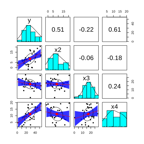
Figure 3.1: The pair plot for each two variables in R
However, with a small sample, as in our case, we should be careful when assessing some results, and the statistic tests are more robust for such kinds of deductions.
# fit the model
model_R <- lm(y~., data=df_R_sample)

# display the summary
result_R <-  tidy(model_R, conf.int = TRUE)
result_R| term | estimate | std.error | statistic | p.value | conf.low | conf.high |
|---|---|---|---|---|---|---|
| (Intercept) | 7.913295 | 3.2101540 | 2.465082 | 0.0206196 | 1.314729 | 14.5118608 |
| x2 | 1.395749 | 0.1413768 | 9.872542 | 0.0000000 | 1.105144 | 1.6863527 |
| x3 | -0.818892 | 0.1443155 | -5.674317 | 0.0000057 | -1.115537 | -0.5222472 |
| x4 | 2.008222 | 0.1636282 | 12.273079 | 0.0000000 | 1.671879 | 2.3445647 |
As we see the estimates are closer to the true parameters. We can also plot the results as follows:
ggplot(result_R,
       aes(
         estimate,
         term,
         xmin = conf.low,
         xmax = conf.high,
         height = 0
       ), na.rm=TRUE) +
  geom_point(size = 2, color = "red") +
  geom_vline(xintercept = 0, lty = 4) +
  geom_errorbarh(color = 'blue') +
  xlab('the estimates') + ylab('the variables') +
  coord_flip() +
  theme_classic()+
  ggsave('conf_R.png', height=5, width=5)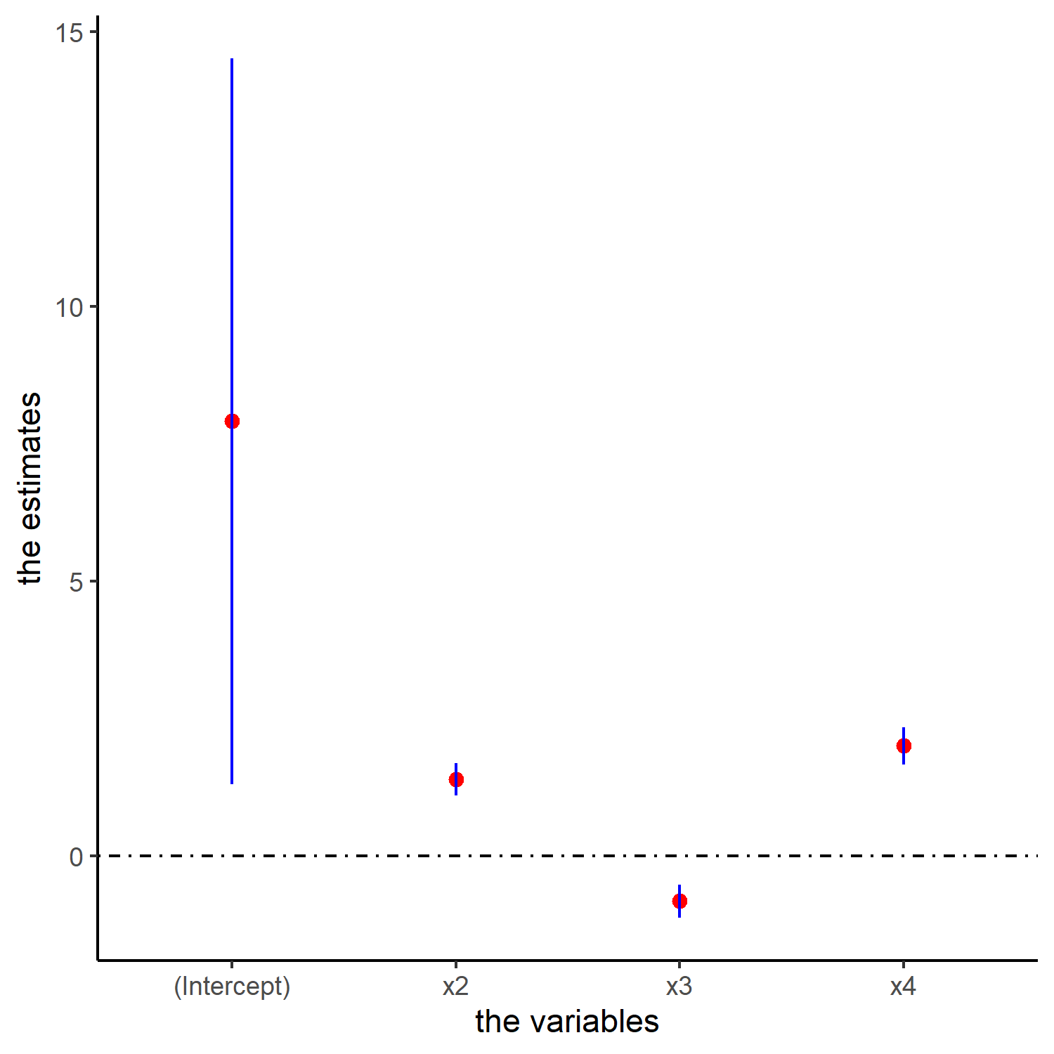
Figure 3.2: The pair plot for each two variables in Python
As we see, the zero value is outside of all the above intervals, which means that all the coefficients are significant.
we generate first the data.
import numpy as np
import statsmodels.formula.api as smf
import pandas as pd

np.random.seed(1)

eps = np.random.normal(0, 5, 100)
X2 = np.random.normal(10,6,100)
X3 = np.random.normal(15, 5, 100)
X4 = np.random.uniform(2,20,100)
Y = 4+1.5*X2-0.6*X3+1.9*X4+eps

df_p = pd.DataFrame({"Y":Y, "X2":X2, "X3":X3, "X4":X4})
Then we select randomly 30 observations as we did in R.
Then we visualize the pair plot.
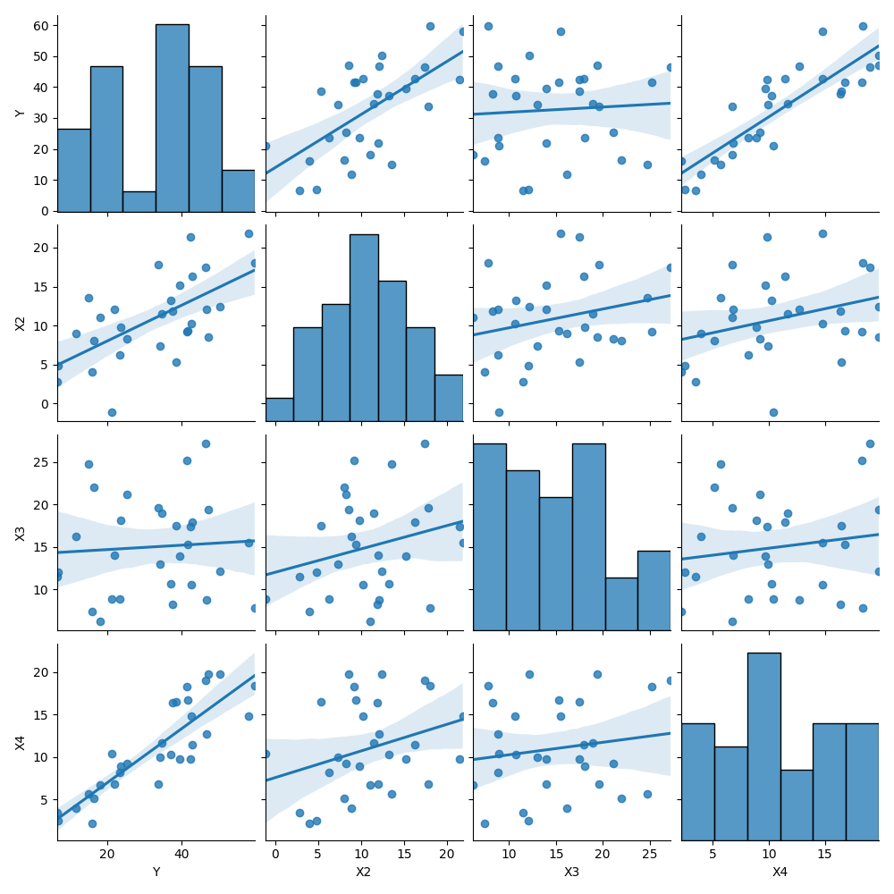
Figure 3.3: The pair plot for each two variables in Python
# fit the model
model_p = smf.ols('Y~X2+X3+X4', data=df_p_sample).fit()
result_p = model_p.summary2().tables[1]

# we remove the index to the columns
result_p.reset_index(inplace=True)
result_p| index | Coef. | Std.Err. | t | P>|t| | [0.025 ] | |
|---|---|---|---|---|---|---|
| Intercept | 3.5782321 | 2.8764907 | 1.243957 | 0.2246140 | -2.3344793 | 9.4909434 |
| X2 | 1.1923048 | 0.1709840 | 6.973194 | 0.0000002 | 0.8408421 | 1.5437674 |
| X3 | -0.4177008 | 0.1537923 | -2.716006 | 0.0115887 | -0.7338254 | -0.1015762 |
| X4 | 2.0368269 | 0.1653634 | 12.317274 | 0.0000000 | 1.6969174 | 2.3767363 |
We can plot the results in python as follows:
import matplotlib.pyplot as plt
# we compute the error bar from the confidence interval
err = model_p.params - model_p.conf_int()[0]
result_p['error'] = err.values

fig= plt.figure(figsize=(15,15))
plt.errorbar(x="index", y= "Coef.",color="red", yerr="error", fmt="o ",
ecolor="blue", data=result_p)
plt.xlabel("the variables")
plt.ylabel("the estimates")
plt.axhline(y=0, linestyle="--")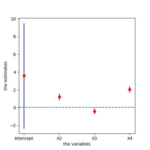
Figure 3.4: the estimates in Python